12 Threats to inference
12.1 Peer review
Research can be flawed. One method that researchers use to reduce these flaws is peer review, in which persons knowledgeable in a research field review a research paper before the research paper can be published in a peer-reviewed journal. The journal’s editor then typically uses the peer reviewer comments to determine whether to publish the paper as is, to request a revised paper, or to reject the paper. The hope is that this peer review process will:
- improve the paper
- provide a signal about the quality of the paper
This signal has multiple parts. The signal can indicate that this paper has sufficient quality to be published, but this signal can also indicate that this paper is important enough or good enough to be published in the journal that is reviewing the paper.
Political science and many other social sciences often use double-blind peer review, in which the author of a submitted paper does not know who the peer reviewers are, and the peer reviewers do not know who the author is. Peer reviewers receive a paper that does not indicate the author’s name, and the author receives peer reviews that do not indicate the peer reviewers’ names. A benefit of double-blind peer review is that the peer reviewers will hopefully evaluate the work instead of evaluating the person who submitted the work; another benefit is that, because the reviewers’ names are kept confidential, the reviewers cannot be punished by the author if the reviewer writes a negative review. A disadvantage of double-blind peer review is that—because the peer reviewers’ names are kept confidential—the peer reviews are sometimes of lower quality than they should be, because the peer reviewers do not get credit for writing a good peer review and are shielded from criticism for writing a bad review.
Natural sciences such as biology and physics typically use single-blind peer review, in which the author does not know who the peer reviewers are, but the peer reviewers know who the author is. One possible advantage of single-blind peer review is in decisions about funding grants. Peer reviewers evaluating the person who submitted the work can help decide whether to trust a researcher with grant money, because peer reviewers might have information about whether the researcher is trustworthy and/or has used grant money wisely in the past and/or does a good and fair job with data analysis. The disadvantage of single-blind peer review is that the peer reviewers might bias their evaluation of the paper because the peer reviewer does not like the paper’s author.
A few journals use triple-blind peer review, which is the same as double-blind review, but with an extra layer of blindness: the journal editor does not know who the author of the paper is. The benefit of this triple-blind peer review is that the editor’s judgment is not influenced by author characteristics. Editors might favor some authors in the decision to publish or in the decision of whom to invite for peer review (if the editor knows which peers provide “easy” reviews). But a drawback of triple-blind peer review is that it is more difficult logistically, so the journal needs an extra layer of review with assistants to help make sure that the editor does not accidentally invite for peer review a co-author of the author of the paper. (Journals typically do not invite peers who have a close connection to the paper’s author, such as co-authors, past advisers, or persons who work in the same department as the author).
Another (relatively uncommon) type of peer review is open peer review, in which the author(s), peer reviewers, and editor(s) all know each others’ names, and the paper and the peer reviews are posted on the internet with names attached to the paper and the reviews. A drawback to open peer review is that the review of the paper might be biased because the reviewer does not like the paper’s author. But advantages of open peer review are that this bias would be more easily detectable and that peer reviewers could be rewarded and/or punished for good reviews and bad reviews.
Blindness in peer review is not always true blindness, because occasionally even under double-blind review, peer reviewers might know who the paper’s author is because, for instance, the author has already publicly presented the paper at a conference. Moreover, the peer reviewers typically do not check the data to make sure that the data has been coded correctly and do not check the statistical analysis to make sure that the statistical analysis has been conducted correctly. Peer review typically involves only the peer reviewers and editors evaluating the research by reading the research paper.
Peer review is therefore not a seal of approval from the scientific community, but instead is more of an attempt to make sure that the paper crosses a minimum threshold of quality for the journal. Peer review does not catch all flaws and biases in research, so it’s a good idea for readers to assess the research on their own.
Let’s discuss a post on the Monkey Cage political science blog at the Washington Post, which published an analysis by Feinberg et al:
We found that counties that had hosted a 2016 Trump campaign rally saw a 226 percent increase in reported hate crimes over comparable counties that did not host such a rally.
One obvious question that this Feinberg et al study did not address was the corresponding percentage increase in hate crimes in counties that hosted a 2016 Hillary Clinton rally. Maybe Trump rallies associated with hate crimes merely because Trump held rallies in large population counties, and large population counties tend to have a larger number of hate crimes, at least partly because large counties have a large number of people who live there. Matthew Lilley and Brian Wheaton ran the numbers and reported in a Reason magazine post from September 2019 that:
Using additional data we collected, we also analyzed the effect of Hillary Clinton’s campaign rallies using the identical statistical framework. The ostensible finding: Clinton rallies contribute to an even greater increase in hate incidents than Trump rallies.
Believe it or not, more than two years after the Lilley and Wheaton criticism was published, the Feinberg et al analysis limited to Trump rallies was published in a peer-reviewed journal.
12.2 Pre-registration
Sometimes researchers don’t publish results from research that they have conducted. One method to reduce selective reporting is pre-registration, in which researchers publicly post ahead of time a plan for the research that they will conduct. This plan might include information such as when the data will be collected, from whom or what the data will be collected, what data will be collected, how the data will be analyzed, and what analyses will be reported. See this link for a sample preregistration.
Let’s discuss some things that can cause an incorrect inference.
12.3 Selection bias
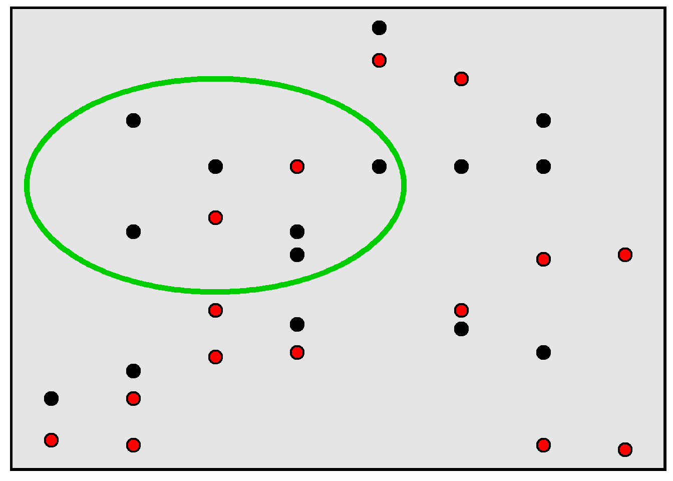
Remember that a population is the set of things of interest for a study, and a sample is the set of things that were studied for the study. Selection bias occurs when a sample is not representative of the population and this causes an incorrect inference about the population. For example, in the rectangle below, 50% of the population of points are red, but, in the sample of points inside the green circle, only 25% of the points are red.
For an example of a potential incorrect inference due to selection bias, suppose that we wanted to estimate the percentage of college students who voted in the most recent election, so we email all college students, asking each student to complete a 50-item survey in which the last item on the survey is an item asking students to report whether they voted in the most recent election. It’s plausible that the percentage of college students who indicated on the survey that they voted in the most recent election is an overestimate of the true percentage of college students who voted in the most recent election, because it’s plausible that the college students who completed the survey are more conscientious on average than other college students and that more conscientious college students are more likely to vote than less conscientious college students are to vote.
Researchers can address an unrepresentative sample by using weights. Researchers can also address missing responses by using imputation, which involves the researcher taking a best guess (or guesses) about what the missing data would have been if the data was not missing. This best guess might be based on data that the researcher has about the observation that had the missing data; for example, if a participant does not indicate their family income, then a researcher might impute a family income for that participant, with the imputed value reflecting the researcher’s best guess at the participant’s income using other data that the researcher knows about the participant, such as the participant’s education level, age, gender, race, and marital status. So if a 40-year-old married Black woman with a college degree does not indicate her family income, we could impute that family income based on the expected family income for a typical 40-year-old married Black woman with a college degree.
12.4 Influential outliers
An outlier is data point that is very different from other data points. Such outliers can cause an incorrect conclusion if the outlier is misleadingly influential.
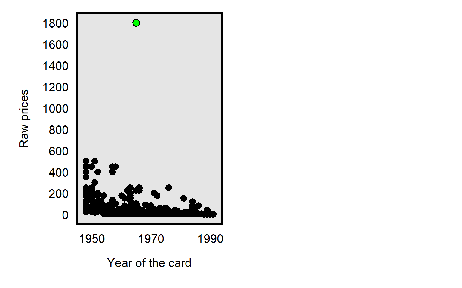
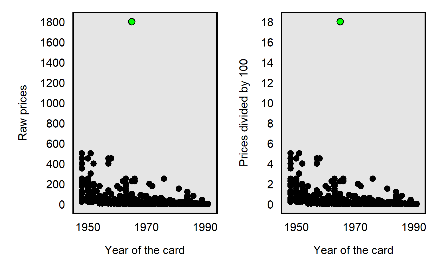
For example, in the dataset for Primm et al 2010 “The Role of Race in Football Card Prices”, the median price for a football card was $3, and the price for all but one football card was $500 or less. However, the football card for Joe Namath was $1,800, which was more than three times as much as the next highest priced card in the dataset, as illustrated in the plot below. So a threat to causal inference would be if Joe Namath’s card is misleadingly influential. Joe Namath is White, so, if our analysis indicated that the cards for White football players were on average priced higher than cards for Black football players were priced, that might be due to unfair bias favoring White players, but we should also assess whether that difference in mean price is due to something distinctive about Joe Namath other than his race.
Researchers have a few ways to deal with outliers, such as:
Conduct the analysis with and without the outlier. For example, for the Joe Namath example of a football card that has an outlier price, we could conduct the analysis including Joe Namath’s card and re-conduct the analysis excluding Joe Namath’s card: if the results are substantially the same, then we can infer that the outlier really doesn’t matter much.
Transform the data so that the outlier is less influential.
One transformation is to reduce the data to categories. For the football card example, instead of measuring the price of football cards to the nearest penny, we could group the cards by price range, such as from 1 cent to 50 cents, 51 cents to 99 cents, $1 to $1.99, and so forth until, say, $300 or more. That way, the Joe Namath card is not all by itself far away from the other cards but is instead in the highest category along with (in this case) 14 other relatively high priced cards. The number of categories and the width of the categories can depend on the amount of data that we have and the usefulness of the categories. This data transformation isn’t ideal, though, because the data transformation loses precision in the measurement, with the $1800 Joe Namath card not being differentiated from the $450 card for Jim Brown or the $300 card for Norm Van Brocklin.
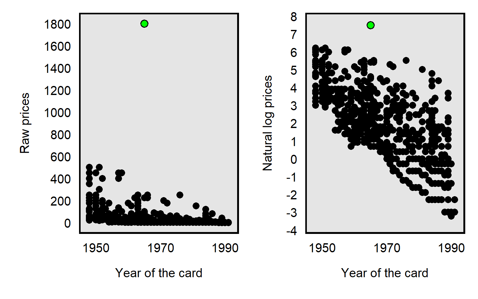
The data transformation that Primm et al 2010 used was the natural log transformation, which pushes numbers together, as illustrated in the plot below, with the Joe Namath card as the green dot:
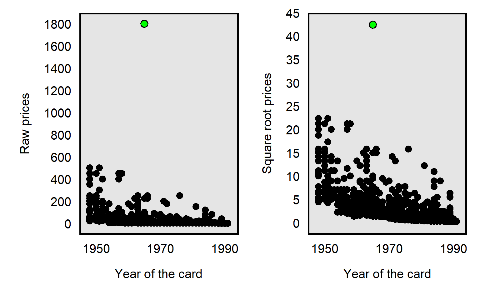
The influence of an outlier can also be reduced by taking the square root the prices, like in the plot below, but, compared to a natural log transformation, the reduction is less extreme for the square root transformation:
It’s possible to divide each card price by, say, 100, which will reduce the price of the Joe Namath card from $1800 to $18. But dividing by 100 will reduce the price of all cards equally relative to each other, so the dividing by 100 doesn’t affect how influential the outlier is:
Sample practice items
Suppose that a dataset contains annual salaries for 100 respondents, with 99 salaries between $10 per year and $200,000 per year and one outlier salary of $20 million per year. We use the measure of respondent annual salary to predict respondent support for raising taxes. Select ALL of the data transformations listed below that would plausibly reduce the influence of the outlier on our estimates:
- dividing the salaries by 100
- taking the natural log of the salaries
- squaring the salaries
- square rooting the salaries
Answer
- taking the natural log of the salaries
- square rooting the salaries
12.5 Measurement error
Measurement error occurs when measurements are incorrect. Below are illustrations:
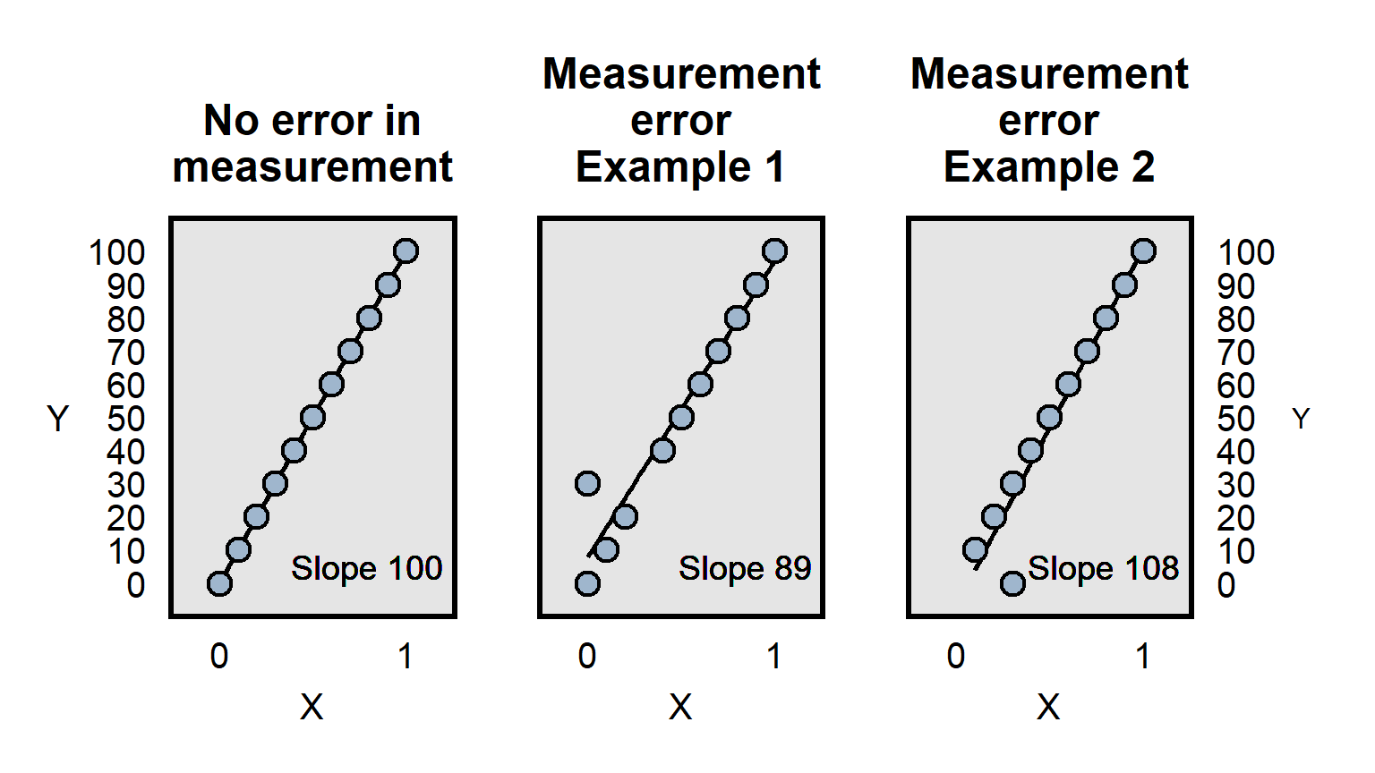
Measurement error can involve incorrect measurement, but imprecise measurement can also be a problem. Imagine, for instance, that a pill really causes participants to lose 10 pounds on average and that we have a measure of participant weight before and after taking the pill. If our measurement of participant weight is merely whether a person is overweight, then we might not have sufficient precision in the measurement of the outcome to detect the true effect of the weight loss pill, if all of the weight loss involves changes such as 250 lbs to 240 lbs, in which both weights are coded as “overweight” and thus there is no change in the measurement.
Differences in measurement precision can be a particular problem for analyses that attempt to compare how well predictors predict an outcome, because a predictor that is measured more precisely will, all else equal, have an advantage in that comparison, because the lack of precision is expected to bias estimates toward zero, as illustrated below:
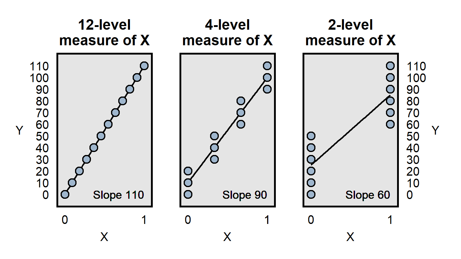
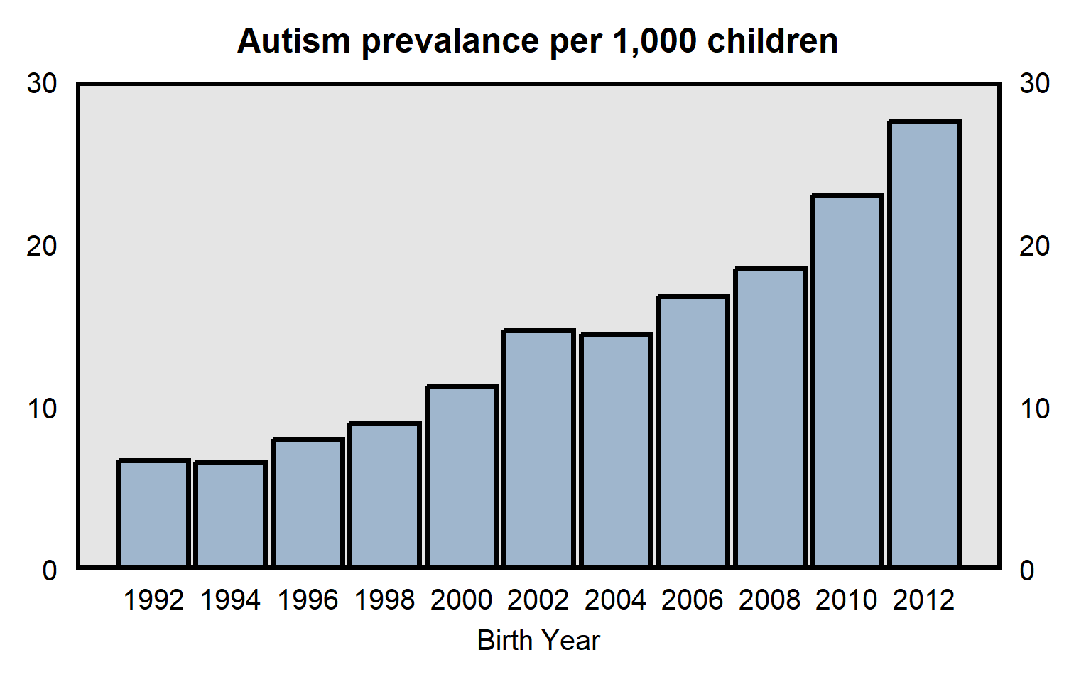
It is useful to consider whether patterns might be influenced by measurement error. For example, data from the Centers for Disease Control and Prevention in the plot below indicates the prevalence of autism among U.S. children born between 1992 and 2012. The substantial increase over time might be due to an increase in the prevalence of autism, but part or all of the increase might be due to changes in the measurement of autism, such as if doctors over time became more likely to diagnose the same set of behaviors as autism.
Sample practice items
Suppose that, over the past ten years, the reported number of burglaries has substantially decreased in Freedonia City. One possible explanation for this is that the prevalence of burglary has dropped. But what else might this be due to?
Answer
One possible response: The decrease in the reported number of burglaries might be due to victims of a burglary being less likely to report the burglary, such as if police over time have become much less likely to sincerely investigate burglaries or much less likely to successfully return stolen goods.12.6 Confounders
The problem of confounding occurs when the association between a predictor and an outcome is due to a third variable, called a confounder.
Consider the van Boven et al 2006 randomized experiment that tested for racial bias, in which participants were randomly shown only one of the photos below and were asked the item below:

Q11. The person in the photograph is holding several items. To what extent to you agree or disagree that this person is looting?

- Strongly Agree
- Moderately Agree
- Slightly Agree
- Neither Agree nor Disagree
- Slightly Disagree
- Moderately Disagree
- Strongly Disagree
The outcome of participant perceptions about whether the person in the photograph is looting could be influenced by the race of the person in the photograph (and thus be influenced by racial bias), but there are other differences between the photographs that confound that inference. For example, compared to the Black person, the White person seems like he is struggling more because he is carrying more items than he can comfortably carry. Even the difference in what is being carried (wine bottle for the White person only) could be a confound that makes it difficult for the experiment to isolate the effect of the race of the person in the photograph.
For another example, suppose that a class has 100 students, and, before the final exam, 20 of the students attend a study session and the other 80 students don’t attend the study session. Suppose that each of the 20 study session students earns a higher score on the final exam than any of the other 80 students earn. It could be that attending the study session caused the higher final exam scores. But it also could be that something else influenced both whether students attended the study session and the students’ scores on the final exam. For example, maybe conscientiousness caused the 20 study session students to attend the study session and to study for the final exam independently of the study session, so that the 20 study session students would have earned a higher scores on the final exam even without the study session.
The problem with multiple manipulations per experimental condition can be subtle. Consider a randomized experiment in which participants in one group are asked to recommend a sentence length for a White man who murdered his wife, and participants in the other group are asked to recommend a sentence length for a Black man who murdered his wife. In this case, only one thing has been explicitly changed: the race of the man who murdered his wife. But, because so many marriages are between persons of the same race, many participants might think that the White man murdered a White woman and that the Black man murdered a Black woman. So if the Black man received a lower mean recommended sentence length than the White man received, we could not tell whether that is because participants punished the White man more severely than the Black man or because the participants thought that taking a White woman’s life deserved a more severe punishment than taking a Black woman’s life deserved.
12.7 Miscontrolling
Flawed statistical control might produce an incorrect inference in at least two ways:
Undercontrolling occurs when the analysis is missing a relevant control. For example, if, at a particular company, men are paid more than women on average, that gender difference in payment might be fair if men work more hours on average than women work, so an analysis that does not control for hours worked might produce an incorrect inference that men at that company are unfairly paid more then women at that company.
Overcontrolling occurs when analysis has too many controls, such as controlling for factors that are “downstream” from the predictor that we are interested in. For example, it might be fair for a company to pay workers more if the worker received an award from the company. So an analysis testing for gender bias in worker pay should control for whether the worker received such an award. But there might be gender bias in the decision about which workers are selected to receive an award, so that controlling for receipt of such awards can produce an incorrect inference about gender bias in worker pay if the awards are a mechanism for gender bias in pay.
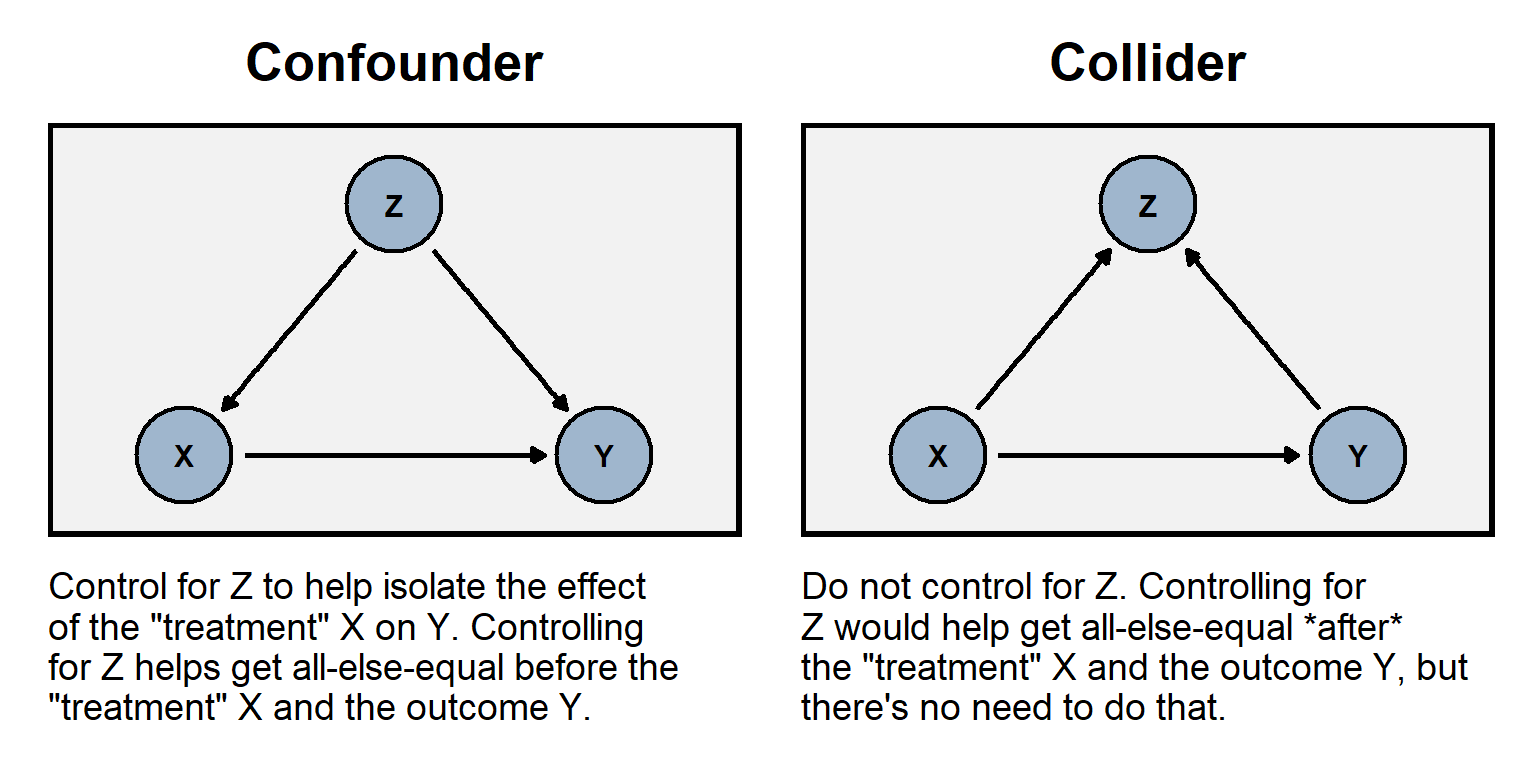
The ideal for control variables is to help get the cases that we are comparing to be equal at the point of the difference in treatment, so that we can estimate the effect of the treatment. Therefore, we want to control for differences that have occurred before the difference in treatment, and we do not want to control for differences that occur because of the difference in treatment.
The plot to the left below illustrates the role of a confounder Z that is “upstream” from a predictor and the outcome; it would be undercontrolling to omit the confounder. The plot to the right below illustrates the role of a collider Z that is “downstream” from a predictor and the outcome; it would be overcontrolling to include the collider.
Like with random assignment error, miscontrolling can bias an estimate to be too low and can bias an estimate to be too high.
For an example of overcontrolling collider bias, consider an analysis of data from a randomized experiment that controls for a factor that is measured after the treatment. For example, suppose that the treatment in an experiment is a campaign ad and that this treatment has two effects: one effect is to make participants more positive about the president, and the other effect is to increase participants’ political interest. Controlling for participant political interest could then bias the estimated effect of the treatment on attitudes about the president. See the table below, with three participants in the control group and three participants in the treatment group, all before receiving the treatment. In this case, the mean political interest is the same in each group, and the mean rating is the same in each group: 70 in the control group, and 70 in the treatment group.
| BEFORE THE TREATMENT | |||
|---|---|---|---|
| Control Group | Treatment Group | ||
| Political Interest | Rating | Political Interest | Rating |
| 4 | 90 | 4 | 90 |
| 3 | 60 | 3 | 60 |
| 3 | 60 | 3 | 60 |
Now check the participants in the table below, after receiving the treatment. The treatment had an effect on the second participant in the treatment group, raising that participant’s political interest to 4 and raising that participant’s rating of the president to 90. The mean of the treatment group has risen to 80.
| AFTER THE TREATMENT | |||
|---|---|---|---|
| Control Group | Treatment Group | ||
| Political Interest | Rating | Political Interest | Rating |
| 4 | 90 | 4 | 90 |
| 3 | 60 | 4 | 90 |
| 3 | 60 | 3 | 60 |
The proper way to analyze the tables is to compare the “after the treatment” control group mean rating of 70 to the “after the treatment” treatment group mean rating of 80 to infer that the treatment has raised the rating by 10 points among these participants. However, if we were to control for participants’ political interest, we would infer that the treatment had no effect, because, at each level of political interest, the mean rating in the treatment group equals the mean rating in the control group.
For a randomized experiment, sometimes researchers control for participant demographics such as race and gender, that are measured before the treatment. This can help reduce uncertainty caused by random assignment error and thus increase the precision of the estimates, which can be a good thing. But researchers sometimes control for participant demographics or other factors that are measured after the treatment, but, as illustrated above, this statistical control can bias estimates if the factors that are measured after the treatment have been affected by the treatment.
Sample practice items
Suppose we test whether variation in X causes variation in Y. Which of the following would be worse to add as a predictor to that regression?
- a variable A that influences X and influences Y
- a variable B that is influenced by X and is influenced by Y
Answer
- a variable B that is influenced by X and is influenced by Y
Suppose that you have a linear regression that attempts to estimate the effect that a predictor has on an outcome. Omitting a control variable that should be included in the regression…
- cannot bias the estimate of the effect of the predictor
- can bias the estimate of the effect of the predictor, but can only bias the estimate toward zero
- can bias the estimate of the effect of the predictor, but can only bias the estimate away from zero
- can bias the estimate of the effect of the predictor, and can bias that estimate toward zero or away from zero
Answer
- can bias the estimate of the effect of the predictor, and can bias that estimate toward zero or away from zero
Suppose that you have a linear regression that attempts to estimate the effect that a predictor has on an outcome. Including a control variable that should not be included in the regression…
- cannot bias the estimate of the effect of the predictor
- can bias the estimate of the effect of the predictor, but can only bias the estimate toward zero
- can bias the estimate of the effect of the predictor, but can only bias the estimate away from zero
- can bias the estimate of the effect of the predictor, and can bias that estimate toward zero or away from zero
Answer
- can bias the estimate of the effect of the predictor, and can bias that estimate toward zero or away from zero
Suppose that, in a particular jurisdiction, Black persons convicted of murder received longer criminal sentences on average, compared to White persons convicted of murder. We want to test whether this on average reflects unfair racial bias in the criminal justice system, which includes persons such as police, prosecutors, judges, and jurors. For each of the following potential control variables, explain whether our analysis should include that control variable:
- the severity of the murder
- the age of the person convicted of murder
- the past criminal history of the person convicted of murder
- the length of sentence that was recommended by the district attorney who represented the state
Answer
So (A) and (C) seem like good controls. For (A), it’s fair that more serious murders cause longer sentences. For (B), if younger murderers receive different sentence lengths than older murderers, then we should control for that, because – if Black murderers and White murderers have different mean ages – we want to isolate the effect of the race of the murderer.
And (C) is a good control theoretically: it seems reasonable that persons with more substantial criminal histories receive longer criminal sentences, all else equal. But this control variable might be contaminated by racial bias among police, if police are unfairly more likely to monitor and/or arrest Black persons than White persons. So we have a good control theoretically but this control is plausibly contaminated by racial bias. The key here is that our analysis is about racial bias among the judges who issue criminal sentences. If we consider it fair for a judge to issue sentences based on the criminal histories of the murderers that the judge is presented with, then it would be appropriate to control for the criminal histories of the murderers.
And (D) is similar, in the sense that racial bias might affect the length of sentence that was recommended by the district attorney.12.8 Reverse causality and reciprocal causality
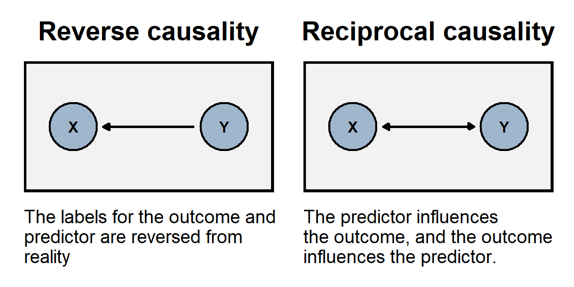
The problem of reverse causality occurs when the association between our predictor and our outcome is because, in reality, the outcome causes variation in the predictor. In other words, we have the direction of causality backwards. For example, if we use the number of police officers per capita in a state to predict the homicide rate in a state, we might conclude that having more police officers causes a state to have a higher homicide rate. But the association might instead be because having a high homicide rates causes a state to hire more police officers.
The problem of reciprocal causality occurs when our predictor and our outcome affect each other. For example, imagine if reading the newspaper caused a person to have higher political knowledge, but having higher political knowledge increased how often a person read the newspaper. We could observe political knowledge associate with how often a person reads the newspaper, but we couldn’t use statistical control to validly estimate how much of that association is due to reading the newspaper.
12.9 Misinterpreting p>0.05
Remember that a p-value is a measure of the strength of evidence that an analysis has provided against a null hypothesis. For political science, a p-value under p=0.05 is sufficient to reject the null hypothesis. A common error of inference is to interpret a p-value that is not under p=0.05 as evidence that the null hypothesis is true. For instance, suppose that we flipped a coin 3 times and got 3 heads and 0 tails. The p-value would be p=0.25 for a test of the null hypothesis that the coin is fair, so that there is not enough evidence to reject the null hypothesis that the coin is fair. But that doesn’t mean that there is enough evidence to infer that the coin is fair: after all, the coin never landed on tails!
For a published example of this, Ono and Zilis 2021 reported on a list experiment that attempted to measure percentages of respondents that agreed with the statement that “When a court case concerns issues like immigration, some Hispanic judges might give biased rulings”. For a test of the null hypothesis that zero percent of Hispanics agreed with that statement, the p-value was not under p=0.05. Ono and Zilis 2021 suggested (p. 4) that:
Hispanics do not believe that Hispanic judges are biased.
However, the estimate from the analysis was that 25% of Hispanics agreed with the statement, so the p-value not being under p=0.05 does not mean that the relatively large 25% estimate should be treated as if it were zero. The figure below presents the 95% confidence interval for this 25% estimate, which suggests that – while the analysis did not provide sufficient evidence that the percentage agreement among Hispanics differs from zero – the analysis also did not provide sufficient evidence that the percentage agreement was zero or was even close to zero. The 95% confidence interval indicates that 0% cannot be excluded as a plausible value, but 50% cannot be excluded as a plausible value, either.
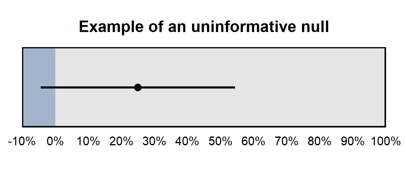
The 95% confidence interval was [-4%, 54%] for the percentage of Hispanics who agreed with the statement, so the analysis did not provide a precise estimate of the percentage of Hispanics who agreed with the statement. This type of imprecise estimate that contains zero can be referred to as an an uninformative null, which means that the analysis did not provide sufficient evidence to reject zero as a plausible value (which makes that a “null” result), and the analysis did not provide sufficient evidence to rule out large estimates as implausible, so the analysis did not provide much information about the what the true number is (which makes the analysis uninformative).
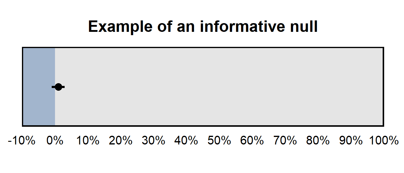
But if the 95% confidence interval has been, say, [-1%, 3%], that would have been an informative null, because – even though the analysis did not provide sufficient evidence to reject zero as a plausible value – the analysis did provide sufficient evidence to rule out large estimates as implausible.
Sample practice items
Of the things in the list below, which would be most useful for assessing whether a null result is an informative null?
- a p-value
- a point estimate
- a 95% confidence interval
Answer
- a 95% confidence interval
Suppose that our outcome is measured on a scale from 0 to 10. Which of the following 95% confidence intervals would be a more informative null, for a treatment effect?
- [-1,2]
- [-40,40]
Answer
- [-1,2]
[-1,2] is a more informative null than [-4,4] is because the ends of [-1,2] is closer to zero.
12.10 Misinterpreting differences in statistical significance
A common bad inference is to infer a difference between estimates merely because the p-value for one estimate falls below a p-value threshold (and is thus “statistically significant”) and the p-value for the other p-value does not fall below that threshold (and is thus not “statistically significant”). This is a bad inference because, to infer something about the difference between estimates, we should have a p-value about that difference in estimates. p-values about each inference aren’t useful for making an inference about the difference between the estimates.
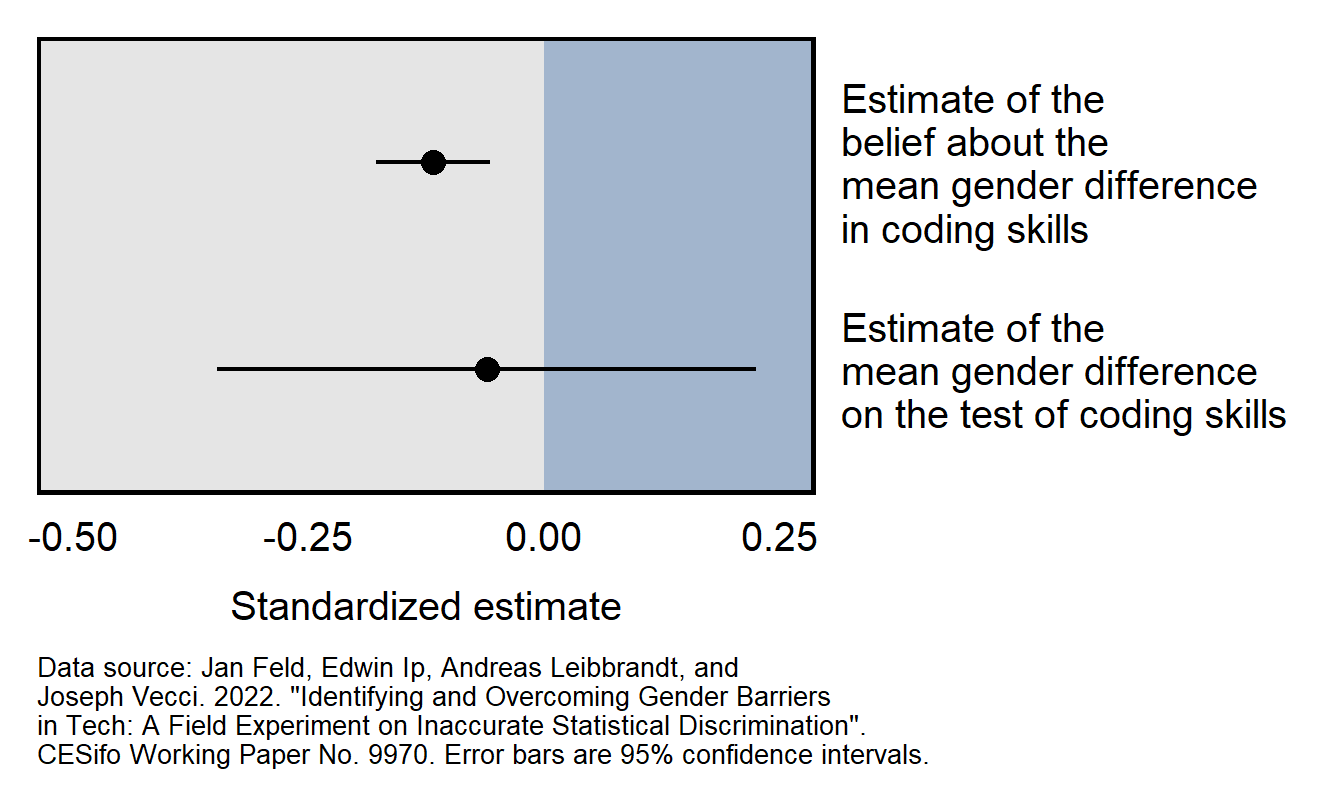
Consider the Feld et al 2022 working paper, which reported that:
We find evidence consistent with inaccurate statistical discrimination: while there are no significant gender differences in performance, employers believe that female programmers perform worse than male programmers.
Results from the working paper are plotted below. The top 95% confidence interval does not cross zero and indicates that there is sufficient evidence to conclude that employers on average thought that the female programmers would perform worse than the male programmers would perform. The bottom 95% confidence interval crosses zero, which means that the analysis did not provide sufficient evidence to conclude that female programmers performed worse than male programmers performed. However, the estimate of the male/female difference in test performance is so imprecise that we can’t conclude with any reasonable confidence that the employers were incorrect in their perception that female programmers would perform worse than the male programmers.
Sample practice items
Suppose that researchers have a sample of men participants and women participants and test the effect of a treatment on the participants. Results provide evidence at p=0.03 that the treatment worked among men, but the p-value is p=0.20 for the test of the effect among women. Is this sufficient evidence to support the conclusion that the treatment was more effective among men than among women?
- Yes: the p-values of p=0.03 and p=0.20 provide sufficient evidence that the treatment worked among men but did not provide sufficient evidence that the treatment worked among women.
- No: p-values do not directly indicate anything about effect sizes, so we cannot conclude based on these p-values that the effect size was larger for men than for women.
Answer
- No: p-values do not directly indicate anything about effect sizes, so we cannot conclude based on these p-values that the effect size was larger for men than for women.
Suppose that, in a linear regression, the coefficient for a predictor of respondent education is 0.20, and the coefficient for a predictor of respondent age is 0.03. Both coefficients are statistically significant. Does this mean that that education has a larger predicted effect on the outcome than age has?
- Yes, because the coefficient for education is larger than the coefficient for age.
- No, because, even though the coefficient for education is larger than the coefficient for age, we need to know the scale of the predictors to assess how big an estimated effect each are.
Answer
B. No, because, even though the coefficient for education is larger than the coefficient for age, we need to know the scale of the predictors to assess how big an estimated effect each are.12.11 Multiple testing
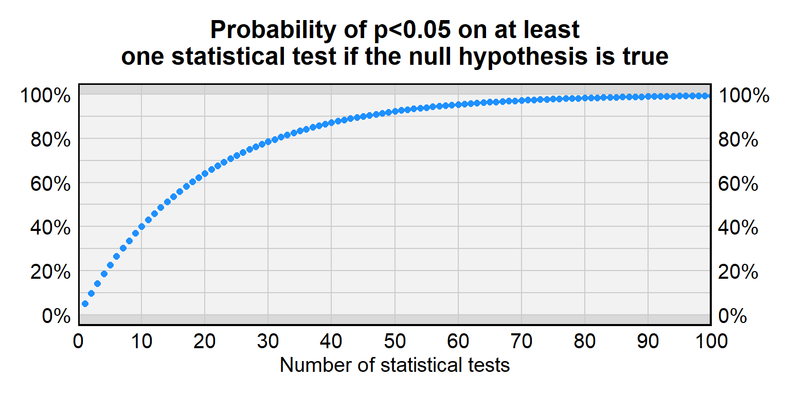
A p-value under p=0.05 sometimes occurs even if a treatment has no effect. In random data, the p-value will be p=0.05 or lower for 5% of statistical tests. But this 5% chance of incorrectly rejecting the null hypothesis is for a single statistical test, and, the more statistical tests we conduct for treatments that have no effect, the higher than chance that at least one of the p-values will be less than p=0.05. The problem of multiple testing is when researchers conduct a lot of statistical tests so that a small p-value for one of the tests becomes more likely to be due to random chance.
For a single test of a true null hypothesis, there is a 5% chance of incorrectly rejecting the null hypothesis and a 95% chance of correctly not rejecting the null hypothesis. For two tests of a true null hypothesis, the probability of correctly not rejecting the null hypothesis both times is \(0.95\times0.95\), which is only about 90%. For ten tests of a true null hypothesis, the probability of correctly not rejecting the null hypothesis all ten times is (0.95)10 which is only about 60%. Below is a table with more information about the false positive rate for a given number of tests.
| Number of tests | Probability of p<0.05 on at least one statistical test if the null hypothesis is true |
|---|---|
| 1 | 5% |
| 2 | 9.7% |
| 3 | 14.3% |
| 5 | 22.6% |
| 10 | 40.1% |
| 20 | 64.1% |
| 50 | 92.3% |
| 100 | 99.4% |
Researchers sometimes adjust p-values to account for this multiple testing problem. The most straightforward adjustment is the Bonferroni correction, in which the p-value threshold is divided by the number of tests that are performed. So, suppose that we conduct four tests of a null hypothesis. If we want to only have a 5% chance of a false positive across all four tests, then, for each test, we use a p-value threshold of p=0.05 divided by 4, which is p=0.0125. Because of this correction, if the null hypothesis is true for all four statistical tests, the probability of a false positive inference will be only 5% across all four tests.
Multiple testing is often a plausible concern about research that reports subgroup analyses without a strong theoretical basis, such as reporting results separately for men and for women if there is no reason to expect that the effect among men to differ from the effect among women. Such subgroup analyses might be due to the researcher searching for a p-value under p=0.05.
12.12 Heterogenous effects
Heterogeneous effects are effects that differ by subgroup, such as if, in a randomized experiment testing for gender bias in candidate preference, Democrats are biased in favor of the female candidate, Republicans are biased in favor of the male candidate. A concern with heterogeneous effects is that the effects offset each other and thus produce an incorrect inference. For example, if, over the full sample, the female candidate is just as likely to be selected as the male candidate is to be selected, we might incorrectly infer that the sample had no gender bias.
Heterogeneous effects can produce overestimates or underestimates of an average effect, depending on whether the sample is representative of the population. For example, suppose that the average effect is +8 among men and is +2 among women. If men and women are equally represented in the population, then the average effect among the population will be +5, which is halfway between +8 and +2. But if men are over-represented in the sample, then the estimated average effect will be larger than the true average effect. And if women are over-represented in the sample, then the estimated average effect will be smaller than the true average effect.
12.13 Participant effects
Participants in a survey sometimes don’t pay attention and might randomly select a response. Researchers can identify respondents who don’t pay attention, by using an attention check such as:
For the next item, no matter what, select “strongly agree”.
For research involving experimental treatments, researchers can use a manipulation check to identify respondents who did not properly receive the treatment. For instance, if the experimental manipulation is the race of a target, then researchers can ask respondents to identify the race of the target that the respondent was asked about. Another type of manipulation check can measure the extent to which a treatment worked. For instance, suppose that we are assessing the influence of happiness on political attitudes, in which the research design for the treatment groups is to instruct a random set of participants to think about something happy and to then ask all participants questions about politics. To check whether participants in the “happy” group are truly more happy than participants in the control group, we might, at the end of the experiment, ask all participants to rate their happiness on a scale from 0 to 10, and then we can check whether the “happy” group has a higher mean level of happiness than the control group has.
Attention checks and manipulation checks are especially useful for assessing the value of a null result in which the analysis does not provide sufficient evidence that a treatment has an effect. In such cases, if a large percentage of participants pass each attention check and if the manipulation check indicates that participants sufficiently received the treatment, then we can credibly conclude that the null result was not due to participant lack of attention. However, if a large percentage of participants fail attention check and/or if the manipulation check indicates that participants did not sufficiently receive the treatment, then the null result should not be interpreted as indicating much about the effect of the treatment.
Let’s discuss three other participant effects:
A demand effect refers to the phenomenon in which a participant’s responses are influenced by what the participant perceives the purpose of the study to be. The bias in a demand effect depends on the participant and the study. For example, if participants think that a researcher is trying to find an association between racial bias and support for Donald Trump, then some participants might insincerely respond in a way to help the researcher find that association, and other participants might insincerely respond in a way to make it harder for the researcher to find that association.
Social desirability is when a participant does not indicate the truth, either by not responding to an item or by providing false information. Such social desirability is a particular concern for measurement of sensitive information, such as a participant’s income or the participant’s level of racism or sexism or a participant’s attitudes about contentious political issues.
Acquiescence bias is the phenomenon that, regardless of the content, some participants are more likely to agree with a statement than to disagree with a statement. Imagine a person who doesn’t care much about Social Security: if that person were asked whether they agree that funding for Social Security should be cut, then that person might agree; but if the same person were asked whether they agree that funding for Social Security should be increased, then that person might also agree. So how a statement is phrased can influence the percentage of participants that agrees with the statement, with the expectation that the percentage of “agree” responses is biased higher than it should be.
12.14 Lack of external validity
Validity is the extent to which a measuring tool measures what the tool is supposed to measure. Internal validity refers to the correctness of a study regarding the sample. External validity refers to the ability to generalize the sample results to a wider population, to a wider range of topics, or to the real world.
For example, suppose that we have students play a first-person shooter game in which they are instructed to shoot only targets who are holding a weapon, and in which the experiment randomizes the race of the targets so that the race of the target is randomly Black or White. The randomization of the race of the target can help us validly conclude whether the participants are racially biased in the way that they played the game. So the game will have a high amount of internal validity for assessing participant racial bias in playing the game. But even if we find evidence of racial bias among our student participants, we cannot credibly generalize that result to police officers, because students are a lot different from police officers, such as the students’ lack of training. And even if the participants were police officers, we could not credibly generalize the video game results to the real world because playing a video game is a lot different than what police officers face in reality. So the game will have a low amount of external validity for assessing racial bias among police officers in the real world.
For an example of a study with high internal validity and high external validity, researchers can conduct an audit study, such as randomly submitting resumes to employers, in which the name on the resume is either a stereotypically Black name or a stereotypically White name. The resumes are identical except for the name on the resume. The researchers then assess whether the resumes with a stereotypically Black name receive a different number of callbacks than the resumes with a stereotypically White name. This study has high internal validity because of the random assignment of names to employers, and the study has high external validity because this is very close (identical, even) to ways that people are called for interviews in the real world.
But even these audit studies aren’t perfect. One concern with resume audit study experiments is that a difference in callback rates by race could be due to social class instead of race, if, for instance, employers are less likely to call back (stereotypically Black) Jamal than (stereotypically White) Brad, but the employers might have been equally likely to call back (stereotypically Black) Jamal and (stereotypically White) Billy Bob. Moreover, audit studies can overestimate racial bias in a job market. Some audit studies match Black applicants and White applicants on all relevant factors such as education and work history that an employer might fairly consider, so that the the employer’s decision will be based on a single factor – race – and not on the potential multitude of factors such as applicant education and work history that employers might typically use in their hiring decisions.
12.15 Violations of statistical assumptions
Statistical tests typically assume that data have particular properties, so, for any statistical test that you perform, it is a good idea to understand these assumptions, check whether the data violate these assumptions, assess the consequences of any violations, and address consequential violations of assumptions.
Let’s discuss a few assumptions of linear regression…
Residuals are normally distributed
Remember that residuals are the differences between the observed values and the predicted values. Correct calculation of p-values for a linear regression is based on the assumption that the residuals are normally distributed. Let’s run a linear regression using data from the ANES 2020 Time Series Study and use the Shapiro–Wilk statistical test (swilk in Stata) to test the null hypothesis that the residuals are normally distributed. For this regression, we will predict respondent ratings about Immigration and Customs Enforcement (ICE):
reg FTICE PID17 FEMALE i.RACE AGE EDUC15, noheader
running D:\OneDrive - IL State University\2-teaching\R for teaching\POL497\prof

> ile.do ...


------------------------------------------------------------------------------
       FTICE |      Coef.   Std. Err.      t    P>|t|     [95% Conf. Interval]
-------------+----------------------------------------------------------------
       PID17 |      6.963      0.139    50.26   0.000        6.692       7.235
      FEMALE |     -2.060      0.600    -3.43   0.001       -3.236      -0.884
             |
        RACE |
2. Black,..  |      6.478      1.131     5.73   0.000        4.260       8.696
3. Hispanic  |     -2.667      1.080    -2.47   0.014       -4.784      -0.550
4. Asian ..  |      5.232      1.671     3.13   0.002        1.956       8.508
5. Native..  |      5.472      2.138     2.56   0.010        1.281       9.663
6. Multip..  |     -0.061      1.684    -0.04   0.971       -3.362       3.239
             |
         AGE |      0.384      0.018    21.54   0.000        0.349       0.419
      EDUC15 |     -1.730      0.278    -6.23   0.000       -2.275      -1.186
       _cons |      9.036      1.630     5.54   0.000        5.840      12.231
------------------------------------------------------------------------------
predict RESIDUALS, residuals
running D:\OneDrive - IL State University\2-teaching\R for teaching\POL497\prof
> ile.do ...
(1,624 missing values generated)swilk RESIDUALS
running D:\OneDrive - IL State University\2-teaching\R for teaching\POL497\prof
> ile.do ...
Shapiro-Wilk W test for normal data
Variable | Obs W V z Prob>z
-------------+------------------------------------------------------
RESIDUALS | 6,656 0.99941 2.043 1.891 0.02929
Note: The normal approximation to the sampling distribution of W'
is valid for 4<=n<=2000.The p-value from the Shapiro–Wilk test is p<0.05, so we can reject the null hypothesis that the residuals are normally distributed, and thus we can conclude that the residuals are not normally distributed. This technically violates an assumption of linear regression. But one concern with statistical tests of an assumption is that a large sample provides enough data for the test to detect even trivial violations of the assumption. So let’s visualize the distribution of residuals:
hist RESIDUALS, normal
running D:\OneDrive - IL State University\2-teaching\R for teaching\POL497\prof

> ile.do ...


(bin=38, start=-83.967087, width=4.4283598)
So the kernel density plot indicates that the residuals are not perfectly normal, but the kernel density plot also indicates that the deviations from normality aren’t extreme.
Let’s also check a pnorm plot (to check for violations of normality in the middle of the distribution of residuals) and a qnorm plot (to check for violations of normality at the ends of the distribution of residuals). For both of these plots, violations will be indicated by deviations from a 45 degree line. In the plots below, there is very little deviation from that line:
pnorm RESIDUALS
running D:\OneDrive - IL State University\2-teaching\R for teaching\POL497\prof

> ile.do ...
qnorm RESIDUALS
running D:\OneDrive - IL State University\2-teaching\R for teaching\POL497\prof

> ile.do ...
By the way, another consideration for statistical tests of assumptions is that small samples will not provide enough information to detect large deviations from the assumption. So consider using visual tests of assumptions.
The variance in the residuals is constant
Linear regression assumes that the variance in the residuals is constant (referred to as “homoskedasticity”). If the variance in the residuals is not constant, this is referred to as “heteroskedasticity”. Let’s use the Breusch-Pagan / Cook-Weisberg test for heteroskedasticity (“estat hettest” in Stata) to test the null hypothesis that the variance in the residuals is constant over predicted values of the outcome:
reg FTICE PID17 FEMALE i.RACE AGE EDUC15, noheader
running D:\OneDrive - IL State University\2-teaching\R for teaching\POL497\prof

> ile.do ...


------------------------------------------------------------------------------
       FTICE |      Coef.   Std. Err.      t    P>|t|     [95% Conf. Interval]
-------------+----------------------------------------------------------------
       PID17 |      6.963      0.139    50.26   0.000        6.692       7.235
      FEMALE |     -2.060      0.600    -3.43   0.001       -3.236      -0.884
             |
        RACE |
2. Black,..  |      6.478      1.131     5.73   0.000        4.260       8.696
3. Hispanic  |     -2.667      1.080    -2.47   0.014       -4.784      -0.550
4. Asian ..  |      5.232      1.671     3.13   0.002        1.956       8.508
5. Native..  |      5.472      2.138     2.56   0.010        1.281       9.663
6. Multip..  |     -0.061      1.684    -0.04   0.971       -3.362       3.239
             |
         AGE |      0.384      0.018    21.54   0.000        0.349       0.419
      EDUC15 |     -1.730      0.278    -6.23   0.000       -2.275      -1.186
       _cons |      9.036      1.630     5.54   0.000        5.840      12.231
------------------------------------------------------------------------------
estat hettest
running D:\OneDrive - IL State University\2-teaching\R for teaching\POL497\prof
> ile.do ...
Breusch-Pagan / Cook-Weisberg test for heteroskedasticity
Ho: Constant variance
Variables: fitted values of FTICE
chi2(1) = 23.19
Prob > chi2 = 0.0000So the statistical test indicates sufficient evidence of heteroskedasticity. Let’s check a visual test for a linear regression that has more than one predictor, by plotting residuals against predicted values of the outcome:
quietly reg FTICE PID17 FEMALE i.RACE AGE EDUC15
running D:\OneDrive - IL State University\2-teaching\R for teaching\POL497\prof

> ile.do ...
predict PREDICTED, xb
running D:\OneDrive - IL State University\2-teaching\R for teaching\POL497\prof
> ile.do ...
(522 missing values generated)rvfplot, mcolor(gs12) addplot(lowess RESIDUALS PREDICTED, color(blue)) yline(0)
running D:\OneDrive - IL State University\2-teaching\R for teaching\POL497\prof
> ile.do ...
There is evidence of a slight violation of the assumption: the blue line indicating the association between the residuals and the predicted values is not at exactly zero over the length of the predicted values of the outcome.
The downward slope of the points might be misleading, because a lot of points fall on top of each other. The reason for the downward slope is the limit of the outcome variable: For example, at a predicted outcome of 20, the residuals range from -20 (for a respondent who was observed to be at 0 but was predicted to be at 20) to +80 (for a respondent who was observed to be at 100 but was predicted to be at 20). But at a predicted outcome of 80, the residuals range from +20 to -80.
A straightforward method to address heteroskedasticity in Stata is to add an option that helps correct standard errors to account for heteroskedasticity, such as “vce(hc3)” (for the acronyms: “variance–covariance matrix of the estimators” and “heteroskedasticity-consistent”):
reg FTICE PID17 FEMALE i.RACE AGE EDUC15, vce(hc3) noheader
running D:\OneDrive - IL State University\2-teaching\R for teaching\POL497\prof

> ile.do ...


------------------------------------------------------------------------------
             |             Robust HC3
       FTICE |      Coef.   Std. Err.      t    P>|t|     [95% Conf. Interval]
-------------+----------------------------------------------------------------
       PID17 |      6.963      0.135    51.42   0.000        6.698       7.229
      FEMALE |     -2.060      0.602    -3.42   0.001       -3.240      -0.880
             |
        RACE |
2. Black,..  |      6.478      1.274     5.09   0.000        3.981       8.974
3. Hispanic  |     -2.667      1.228    -2.17   0.030       -5.074      -0.260
4. Asian ..  |      5.232      1.673     3.13   0.002        1.952       8.512
5. Native..  |      5.472      2.293     2.39   0.017        0.977       9.967
6. Multip..  |     -0.061      1.819    -0.03   0.973       -3.627       3.504
             |
         AGE |      0.384      0.018    21.63   0.000        0.350       0.419
      EDUC15 |     -1.730      0.287    -6.03   0.000       -2.293      -1.168
       _cons |      9.036      1.669     5.42   0.000        5.765      12.307
------------------------------------------------------------------------------
See, for example, this post at Data Colada.
Handling violations of assumptions
If an assumption of a statistical test is violated, a few options are:
ignore the violation, if the violation is not consequential
transform the variables in some way to reduce or eliminate the violation
use another statistical method that has less consequential violations