11 Moderators
11.1 Moderators
A moderator affects the strength of an association between a predictor and an outcome.
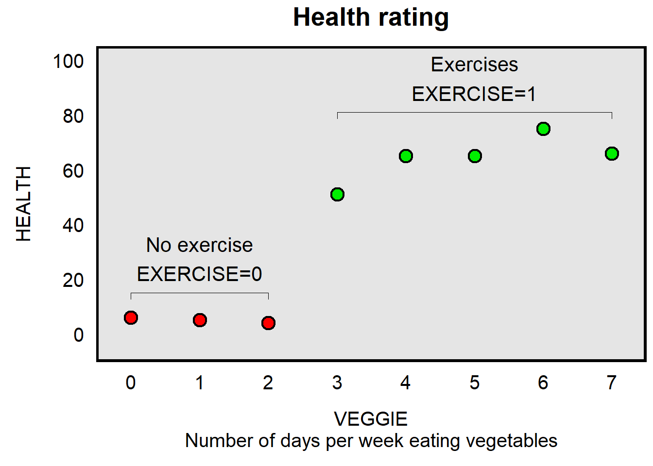
Let’s use a visual example. The plot below presents data for eight persons. The x-axis is a variable called VEGGIE, which indicates how many days per week that each of the eight persons eats vegetables, the y-axis is HEALTH, which indicates a rating about how healthy the person is, and the color of the dots indicates whether the person exercises, with a red dot indicating that the person does not exercise and a green dot indicating that the person exercises (with a variable called EXERCISE).
One way to model the association between VEGGIE and HEALTH is to merely draw a line of best fit through all of the points, like below, and to not incorporate information from the EXERCISE variable.
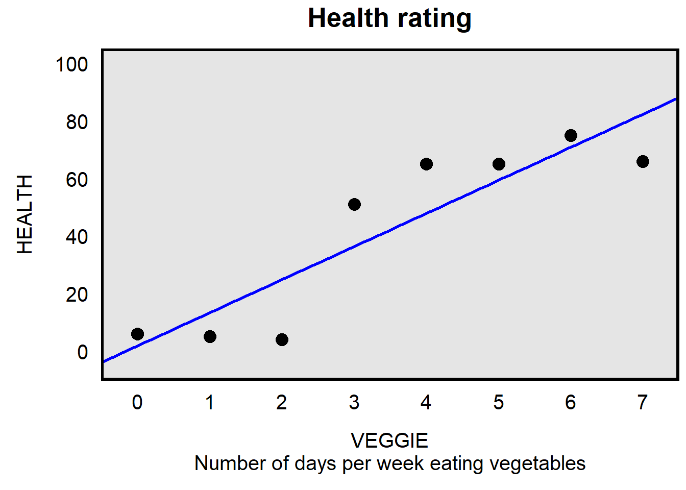
For the regression above, the line of best fit is:
HEALTH = 1.83 + 11.51*VEGGIE
Another way to model the association between VEGGIE and HEALTH is to draw a line of best fit through all of the points, but to control for whether a person exercises. This line of best fit has the same slope, regardless of whether a person exercises or does not exercise, but the height of the line of best fit depends on whether a person exercises or does not exercise. For this equation, there is one slope for VEGGIE, but the predicted outcome of HEALTH also depends on whether EXERCISE is coded 1 or 0.
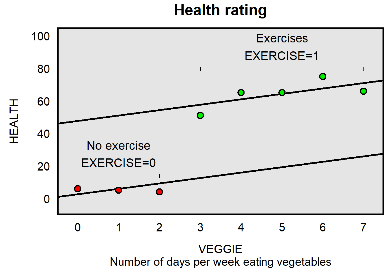
For the regression above, the line of best fit is:
HEALTH = 1.83 + 3.17*VEGGIE + 46.73*EXERCISE
Another way to model the association between VEGGIE and HEALTH is to draw a line of best fit through the EXERCISE=0 points and another line of best fit through the EXERCISE=1 points.
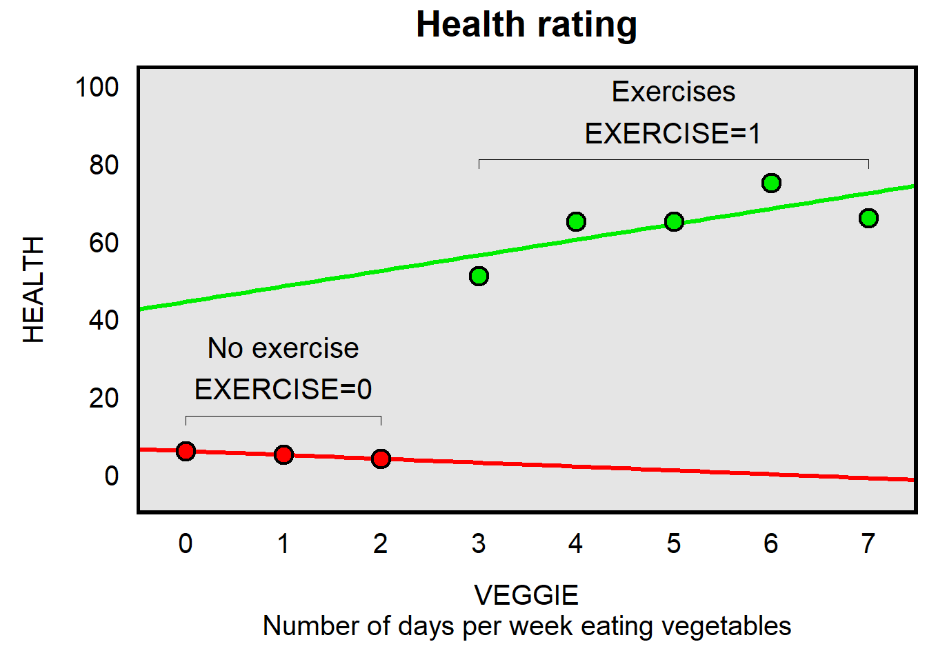
The linear regression output for this “interaction” model is below:
reg HEALTH i.EXERCISE##c.VEGGIE, noheader
running D:\OneDrive - IL State University\2-teaching\R for teaching\POL497\prof

> ile.do ...


------------------------------------------------------------------------------
      HEALTH |      Coef.   Std. Err.      t    P>|t|     [95% Conf. Interval]
-------------+----------------------------------------------------------------
  1.EXERCISE |      38.40      10.93     3.51   0.025         8.06       68.74
      VEGGIE |      -1.00       4.11    -0.24   0.820       -12.41       10.41
             |
    EXERCISE#|
    c.VEGGIE |
          1  |       5.00       4.50     1.11   0.329        -7.50       17.50
             |
       _cons |       6.00       5.31     1.13   0.321        -8.74       20.74
------------------------------------------------------------------------------
For the regression above, the line of best fit is:
HEALTH = 6 + 38.40*EXERCISE + -1*VEGGIE + 5*VEGGIE*EXERCISE
This equation is a bit trickier to interpret, but here goes, for a linear regression with an interaction between a categorical predictor that has two levels (0 and 1) and a continuous predictor:
- Like with any linear regression, the constant/intercept is the predicted outcome when all predictors are zero.
- The continuous predictor by itself is the slope of the continuous predictor when the categorical predictor is zero.
- The categorical predictor by itself is the slope of the categorical predictor when the continuous predictor is zero.
- The interaction term indicates how much the slope of the continuous predictor when the categorical predictor is 1 differs from the slope of the continuous predictor when the categorical predictor is 0.
So, for the VEGGIE*EXERCISE interaction equation:
- The constant/intercept of 6 is the predicted HEALTH when VEGGIE is 0 and EXERCISE is 0.
- The VEGGIE coefficient of -1 indicates the association between VEGGIE and EXERCISE when EXERCISE is 0.
- The EXERCISE coefficient of 38.40 indicates the association between VEGGIE and HEALTH when VEGGIE is 0.
- The VEGGIE*EXERCISE coefficient of 5 indicates how much the slope of the continuous predictor when the categorical predictor is 1 differs from the slope of the continuous predictor when the categorical predictor is 0. This is tricky, because the 5 is not the slope of VEGGIE when EXERCISE is 1, but is instead the difference between slopes. The slope of VEGGIE when EXERCISE is 1 is therefore 5 + -1, which is 4.
11.2 Moderators in Stata
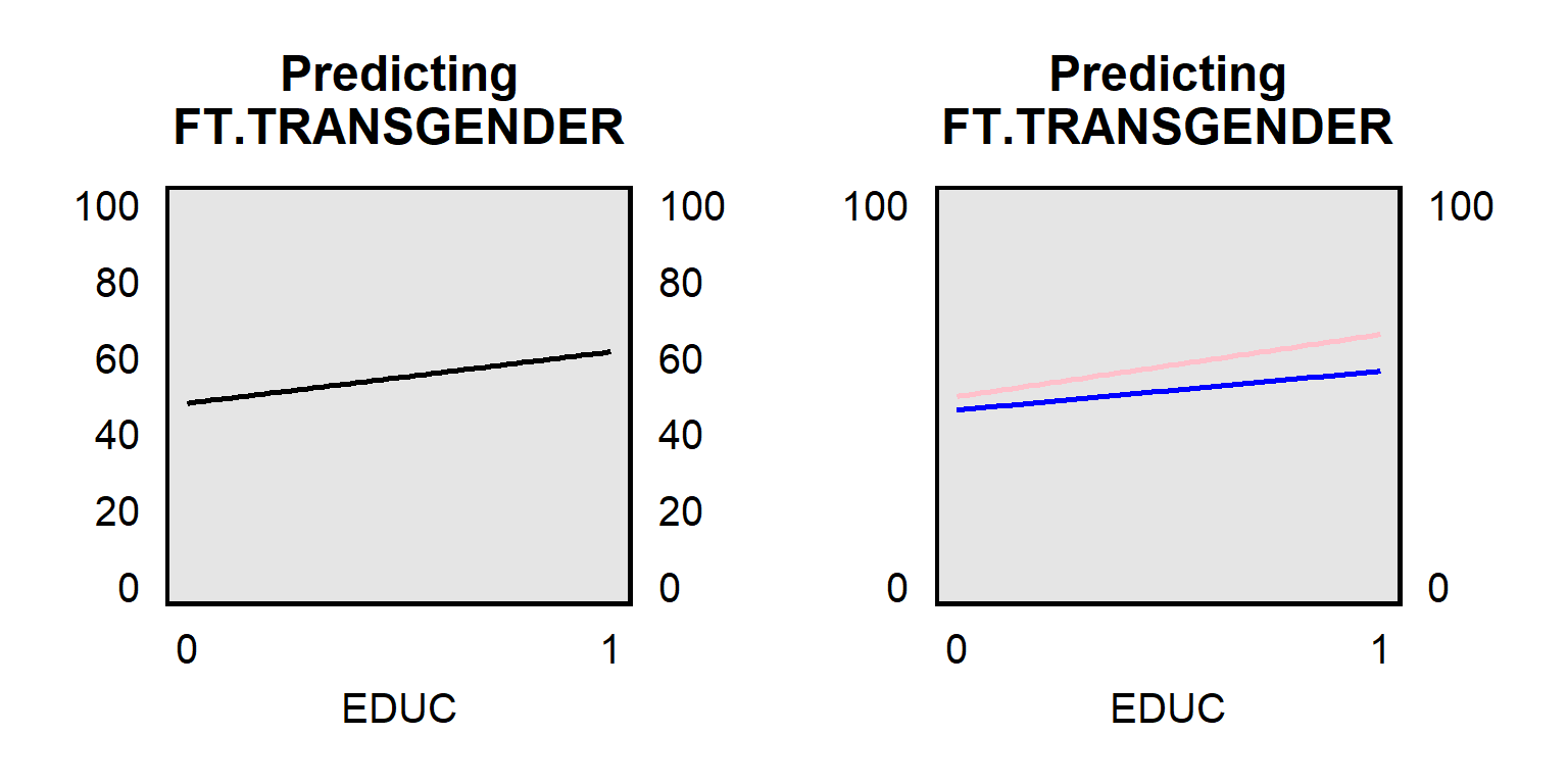
Let’s check data from the ANES 2016 Time Series Study for the association between an outcome of respondent feeling thermometer ratings about transgender persons (FT.TRANSGENDER) coded from 0 for very cold to 100 for very warm and a predictor of respondent education (EDUC), coded 0 for less than a high school education, 0.2 for a high school education, 0.4 for some college, 0.6 for a two year associate’s degree, 0.8 for a four-year bachelor’s degree, and 1 for a post-graduate degree. The panel on the left below plots the association between FT.TRANSGENDER and EDUC among all respondents, and the panel on the right below plots the association between FT.TRANSGENDER and EDUC among female respondents (top pink line) and among male respondents (bottom blue line). The slope for female respondents differs from the slope for male respondents, indicating that gender is a moderator between FT.TRANSGENDER and EDUC.
The first set of linear regression output below is from Stata and is for only female respondents:
reg FTTRANSGENDER EDUC if MALE==0, noheader
running D:\OneDrive - IL State University\2-teaching\R for teaching\POL497\prof
> ile.do ...
------------------------------------------------------------------------------
FTTRANSGEN~R | Coef. Std. Err. t P>|t| [95% Conf. Interval]
-------------+----------------------------------------------------------------
EDUC | 16.28 2.05 7.93 0.000 12.25 20.31
_cons | 49.70 1.32 37.76 0.000 47.12 52.28
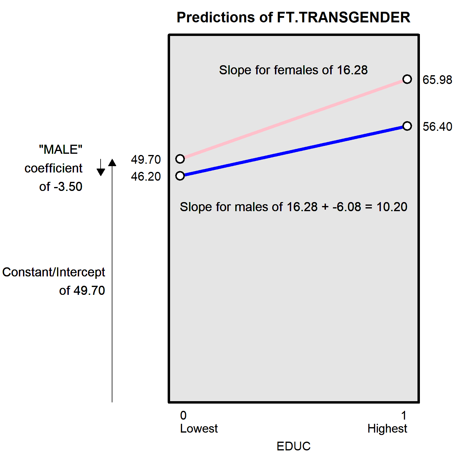
------------------------------------------------------------------------------The linear regression output indicates that the predicted rating about transgender persons was 49.70 for female respondents with the lowest level of education and that this predicted rating increases by 16.28 points for a one-unit increase in EDUC. Because EDUC was coded from 0 for lowest education to 1 for highest education, female respondents at the highest level of education are predicted to rate transgender persons at 49.70 + 16.28, or 65.98.
The linear regression output below uses EDUC to predict ratings about transgender persons, among male respondents. The output indicates that the predicted rating about transgender persons was 46.20 for male respondents with the lowest level of education and that this predicted rating increases by 10.20 points for a one-unit increase in EDUC. Because EDUC was coded from 0 for lowest education to 1 for highest education, male respondents at the highest level of education are predicted to rate transgender persons at 46.20 + 10.20, or 56.40.
reg FTTRANSGENDER EDUC if MALE==1, noheader
running D:\OneDrive - IL State University\2-teaching\R for teaching\POL497\prof

> ile.do ...


------------------------------------------------------------------------------
FTTRANSGEN~R |      Coef.   Std. Err.      t    P>|t|     [95% Conf. Interval]
-------------+----------------------------------------------------------------
        EDUC |      10.20       2.06     4.95   0.000         6.16       14.24
       _cons |      46.20       1.32    35.11   0.000        43.62       48.78
------------------------------------------------------------------------------
The difference in slopes – 16.28 for female respondents, and 10.20 for male respondents – suggests that the association between EDUC and FTTRANSGENDER for female respondents might differ from the corresponding association association between EDUC and FTTRANSGENDER among male respondents. The linear regression below uses an interaction term to test the null hypothesis that the difference in these associations is zero. The double hashtag (##) tells Stata to interact the variables on either side of the double hashtag. The “i.” prefix tells Stata to treat the corresponding variable as a categorical “indicator” variable, and the “c.” prefix tells Stata to treat the corresponding variable as a continuous variable.
In the regression, the predictor for this interaction is i.MALE#c.EDUC, which is an indication of how much the association between EDUC and FTTRANSGENDER among male respondents differs from the association between EDUC and FTTRANSGENDER among female respondents. Importantly, the -6.08 coefficient on i.MALE#c.EDUC does not indicate that the EDUC association is negative among male respondents. Instead, the negative coefficient on i.MALE#c.EDUC merely indicates that the association between EDUC and FTTRANSGENDER among male respondents is lower than the association between EDUC and FTTRANSGENDER among female respondents. The i.MALE#c.EDUC p-value of p=0.037 indicates that there is sufficient evidence at p<0.05 to conclude at the conventional level in political science the association between EDUC and FTTRANSGENDER among male respondents differs from the association between EDUC and FTTRANSGENDER among female respondents.
reg FTTRANSGENDER i.MALE##c.EDUC, noheader
running D:\OneDrive - IL State University\2-teaching\R for teaching\POL497\prof

> ile.do ...


------------------------------------------------------------------------------
FTTRANSGEN~R |      Coef.   Std. Err.      t    P>|t|     [95% Conf. Interval]
-------------+----------------------------------------------------------------
      1.MALE |      -3.50       1.86    -1.88   0.060        -7.15        0.15
        EDUC |      16.28       2.03     8.03   0.000        12.31       20.26
             |
 MALE#c.EDUC |
          1  |      -6.08       2.91    -2.09   0.037       -11.79       -0.37
             |
       _cons |      49.70       1.30    38.25   0.000        47.15       52.24
------------------------------------------------------------------------------
Let’s discuss the remainder of the coefficients estimates in the interaction regression. The individual predictors that make up the interaction term are called constituent terms (or constitutive terms). These constituent terms are interpreted with the other terms in the interaction set to zero. So the coefficient of 16.28 for the EDUC constituent term indicates that the estimated effect of education is 16.28 when MALE is set to zero. In other words, 16.28 is the predicted change in the FTTRANSGENDER outcome among female respondents, given a one-unit change in EDUC.
The coefficient of -3.50 for MALE is the predicted change in the FTTRANSGENDER outcome due to a one-unit change in MALE when EDUC is zero, which, in this regression, is the predicted difference in FTTRANSGENDER between male respondents at the lowest level of EDUC and female respondents at the lowest level of EDUC. The interpretation of MALE cannot be a general difference between male respondents and female respondents in this regression, because this regression has an interaction term, which means that the difference between male respondents and female respondents can differ depending on the level of EDUC.
The constant/intercept of 49.70 is the predicted FTTRANSGENDER outcome when EDUC and MALE are both set to zero, which in this regression is the predicted outcome among female respondents who have the lowest level of EDUC.
Let’s plot the data for the regressions so far:
The regression output that includes the constant/intercept, EDUC, MALE, and the interaction of EDUC and MALE indicates the p-value for the EDUC slope (which is for female respondents), and indicates the p-value for how much the EDUC slope among male respondents differs from the EDUC slope among female respondents. But the regression output does not indicate the p-value for the EDUC slope among male respondents. For that, it’s possible to re-run the regression using predictors of EDUC, FEMALE, and the interaction of EDUC and FEMALE:
gen FEMALE = 1 - MALE
running D:\OneDrive - IL State University\2-teaching\R for teaching\POL497\prof

> ile.do ...
tab MALE FEMALE, mi
running D:\OneDrive - IL State University\2-teaching\R for teaching\POL497\prof
> ile.do ...
| FEMALE
MALE | 0 1 | Total
-----------+----------------------+----------
0 | 0 1,858 | 1,858
1 | 1,654 0 | 1,654
-----------+----------------------+----------
Total | 1,654 1,858 | 3,512 So the output below has a line for EDUC that represents the slope of EDUC among male respondents.
reg FTTRANSGENDER i.FEMALE##c.EDUC, noheader
running D:\OneDrive - IL State University\2-teaching\R for teaching\POL497\prof

> ile.do ...


------------------------------------------------------------------------------
FTTRANSGEN~R |      Coef.   Std. Err.      t    P>|t|     [95% Conf. Interval]
-------------+----------------------------------------------------------------
    1.FEMALE |       3.50       1.86     1.88   0.060        -0.15        7.15
        EDUC |      10.20       2.09     4.88   0.000         6.10       14.30
             |
      FEMALE#|
      c.EDUC |
          1  |       6.08       2.91     2.09   0.037         0.37       11.79
             |
       _cons |      46.20       1.34    34.59   0.000        43.58       48.81
------------------------------------------------------------------------------
But the p-value for the slope of EDUC among male respondents could also have been calculated using the lincom (linear combination) command in Stata. Let’s use the initial interaction regression, and then use a lincom command that tells Stata to add the slope of EDUC among female respondents to the difference in how much the slope among male respondents differs from the slope among female respondents:
reg FTTRANSGENDER i.MALE##c.EDUC, noheader
running D:\OneDrive - IL State University\2-teaching\R for teaching\POL497\prof

> ile.do ...


------------------------------------------------------------------------------
FTTRANSGEN~R |      Coef.   Std. Err.      t    P>|t|     [95% Conf. Interval]
-------------+----------------------------------------------------------------
      1.MALE |      -3.50       1.86    -1.88   0.060        -7.15        0.15
        EDUC |      16.28       2.03     8.03   0.000        12.31       20.26
             |
 MALE#c.EDUC |
          1  |      -6.08       2.91    -2.09   0.037       -11.79       -0.37
             |
       _cons |      49.70       1.30    38.25   0.000        47.15       52.24
------------------------------------------------------------------------------
lincom EDUC + 1.MALE#c.EDUC
running D:\OneDrive - IL State University\2-teaching\R for teaching\POL497\prof
> ile.do ...
( 1) EDUC + 1.MALE#c.EDUC = 0
------------------------------------------------------------------------------
FTTRANSGEN~R | Coef. Std. Err. t P>|t| [95% Conf. Interval]
-------------+----------------------------------------------------------------
(1) | 10.20 2.09 4.88 0.000 6.10 14.30
------------------------------------------------------------------------------Sample practice items
Let’s use the data below, from the ANES 2016 Time Series Study:
reg FTFEMINISTS i.MALE##c.EDUC, noheader
running D:\OneDrive - IL State University\2-teaching\R for teaching\POL497\prof

> ile.do ...


------------------------------------------------------------------------------
 FTFEMINISTS |      Coef.   Std. Err.      t    P>|t|     [95% Conf. Interval]
-------------+----------------------------------------------------------------
      1.MALE |      -1.40       1.78    -0.79   0.430        -4.88        2.08
        EDUC |      18.13       1.93     9.40   0.000        14.35       21.92
             |
 MALE#c.EDUC |
          1  |     -12.34       2.78    -4.44   0.000       -17.78       -6.89
             |
       _cons |      49.78       1.24    40.26   0.000        47.35       52.20
------------------------------------------------------------------------------
Based on the output, what is the association between EDUC and FTFEMINISTS, among female respondents?
- 18.13
- 18.13 + -1.40
- 18.13 + -12.34
- -12.34
Answer
- 18.13
Based on the output, what is the association between EDUC and FTFEMINISTS, among male respondents?
- 18.13
- 18.13 + -1.40
- 18.13 + -12.34
- -12.34
Answer
- 18.13 + -12.34
Based on the output, the constant/intercept of 49.78 indicates the predicted outcome among…
- male respondents on average
- female respondents on average
- male respondents coded 0 for EDUC
- female respondents coded 0 for EDUC
Answer
- female respondents coded 0 for EDUC
11.3 Moderators or separate regressions?
An alternative to running a linear regression that has an interaction between two predictors is to run separate linear regressions for each predictor and to then test for differences in the slopes of the predictors across the regressions. This choice between one regression and two repressions matters if the regression contains control variables and this can affect the moderator predictors, because – for a linear regression with a moderator – the estimates for the control variables are averaged across the predictors. However, for separate linear regressions, the estimates for the control variables are limited to each separate regressions.
Let’s illustrate this with a linear regression on data from the ANES 2016 Time Series Study, predicting ratings about Black Lives Matter, using a predictor for whether a respondent was White or not White, a predictor for respondent age, and a predictor for whether the respondent has a college degree. This regression interacts the predictors for race and age.
reg FTBLM i.WHITE##c.AGE COLLEGE, noheader
running D:\OneDrive - IL State University\2-teaching\R for teaching\POL497\prof

> ile.do ...


------------------------------------------------------------------------------
       FTBLM |      Coef.   Std. Err.      t    P>|t|     [95% Conf. Interval]
-------------+----------------------------------------------------------------
     1.WHITE |    -28.676      3.411    -8.41   0.000      -35.364     -21.988
         AGE |     -0.189      0.060    -3.17   0.002       -0.306      -0.072
             |
 WHITE#c.AGE |
          1  |      0.130      0.069     1.89   0.059       -0.005       0.265
             |
     COLLEGE |      2.062      1.047     1.97   0.049        0.010       4.114
       _cons |     72.708      2.861    25.41   0.000       67.099      78.317
------------------------------------------------------------------------------
In the above regression, the coefficient for COLLEGE is 2.062, which is a weighted average of the coefficients for COLLEGE across racial groups, as indicated in the output for the two regressions below, in which the coefficient for COLLEGE is 4.679 among White respondents and is -4.994 among the smaller sample of non-White respondents.
reg FTBLM AGE COLLEGE if WHITE==1, noheader
running D:\OneDrive - IL State University\2-teaching\R for teaching\POL497\prof

> ile.do ...


------------------------------------------------------------------------------
       FTBLM |      Coef.   Std. Err.      t    P>|t|     [95% Conf. Interval]
-------------+----------------------------------------------------------------
         AGE |     -0.056      0.035    -1.61   0.108       -0.124       0.012
     COLLEGE |      4.679      1.236     3.79   0.000        2.255       7.103
       _cons |     42.385      2.027    20.91   0.000       38.410      46.360
------------------------------------------------------------------------------
reg FTBLM AGE COLLEGE if WHITE==0, noheader
running D:\OneDrive - IL State University\2-teaching\R for teaching\POL497\prof
> ile.do ...
------------------------------------------------------------------------------
FTBLM | Coef. Std. Err. t P>|t| [95% Conf. Interval]
-------------+----------------------------------------------------------------
AGE | -0.168 0.058 -2.89 0.004 -0.281 -0.054
COLLEGE | -4.994 1.946 -2.57 0.010 -8.813 -1.175
_cons | 74.888 2.814 26.61 0.000 69.365 80.411
------------------------------------------------------------------------------Let’s use a lincom command to test whether the -0.056 coefficient for AGE in the regression among White respondents equals the -0.168 coefficient for AGE in the regression among non-White respondents.
quietly reg FTBLM AGE COLLEGE if WHITE==1
estimates store WHITE
quietly reg FTBLM AGE COLLEGE if WHITE==0
estimates store NONWHITE
suest WHITE NONWHITE
running D:\OneDrive - IL State University\2-teaching\R for teaching\POL497\prof

> ile.do ...


Simultaneous results for WHITE, NONWHITE

                                                Number of obs     =      3,464

------------------------------------------------------------------------------
             |               Robust
             |      Coef.   Std. Err.      z    P>|z|     [95% Conf. Interval]
-------------+----------------------------------------------------------------
WHITE_mean   |
         AGE |     -0.056      0.036    -1.57   0.117       -0.125       0.014
     COLLEGE |      4.679      1.228     3.81   0.000        2.273       7.086
       _cons |     42.385      2.067    20.50   0.000       38.334      46.436
-------------+----------------------------------------------------------------
WHITE_lnvar  |
       _cons |      6.851      0.019   354.66   0.000        6.813       6.889
-------------+----------------------------------------------------------------
NONWHITE_m~n |
         AGE |     -0.168      0.058    -2.87   0.004       -0.282      -0.053
     COLLEGE |     -4.994      1.924    -2.60   0.009       -8.765      -1.223
       _cons |     74.888      2.884    25.97   0.000       69.236      80.540
-------------+----------------------------------------------------------------
NONWHITE_l~r |
       _cons |      6.767      0.042   159.70   0.000        6.683       6.850
------------------------------------------------------------------------------
lincom [WHITE_mean]AGE - [NONWHITE_mean]AGE
running D:\OneDrive - IL State University\2-teaching\R for teaching\POL497\prof
> ile.do ...
( 1) [WHITE_mean]AGE - [NONWHITE_mean]AGE = 0
------------------------------------------------------------------------------
| Coef. Std. Err. z P>|z| [95% Conf. Interval]
-------------+----------------------------------------------------------------
(1) | 0.112 0.068 1.64 0.102 -0.022 0.246
------------------------------------------------------------------------------So the slope for AGE among White respondents is 0.112 higher than the slope for AGE among non-White respondents, but the p-value of p=0.102 does not provide enough information at the conventional level in political science that these slopes differ from each other. That’s the same inference as from the regression that interacted AGE and WHITE, but the difference in slope and the corresponding p-value (0.130 and p=0.059) differed from the slope and p-value from the lincom command.
11.4 Interacting with more than two categories
Let’s run a regression that predicts respondent ratings about Black Lives Matter, interacting respondent education level (coded from 0 for less than a high school education to 5 for a graduate degree) and a three-level measure of respondent partisanship (coded Democrat, Independent, and Republican):
reg FTBLM i.PARTY3##c.EDUC, noheader
running D:\OneDrive - IL State University\2-teaching\R for teaching\POL497\prof

> ile.do ...


------------------------------------------------------------------------------
       FTBLM |      Coef.   Std. Err.      t    P>|t|     [95% Conf. Interval]
-------------+----------------------------------------------------------------
      PARTY3 |
2. Republ..  |    -34.844      2.541   -13.71   0.000      -39.825     -29.862
3. Indepe..  |    -16.977      2.336    -7.27   0.000      -21.557     -12.397
             |
        EDUC |      1.229      0.498     2.47   0.014        0.251       2.206
             |
      PARTY3#|
      c.EDUC |
2. Republ..  |     -1.570      0.782    -2.01   0.045       -3.104      -0.036
3. Indepe..  |     -1.363      0.732    -1.86   0.062       -2.798       0.071
             |
       _cons |     63.843      1.643    38.86   0.000       60.621      67.064
------------------------------------------------------------------------------
The 1.229 coefficient for EDUC is the slope of EDUC among the omitted category of Democrats. The -1.570 coefficient for the interaction of EDUC and Republican is how much the slope of EDUC among Republicans differs from the slope of EDUC among the omitted category of Democrats, so – for Republicans – that slope is 1.229 + -1.570, or -0.341. The -1.363 coefficient for the interaction of EDUC and Independent is how much the slope of EDUC among Independents differs from the slope of EDUC among the omitted category of Democrats, so – for Independents – that slope is 1.229 + -1.363, or -0.134. Let’s check the slope for Independents by having Stata use Independents as the omitted category:
reg FTBLM ib3.PARTY3##c.EDUC, noheader
running D:\OneDrive - IL State University\2-teaching\R for teaching\POL497\prof

> ile.do ...


------------------------------------------------------------------------------
       FTBLM |      Coef.   Std. Err.      t    P>|t|     [95% Conf. Interval]
-------------+----------------------------------------------------------------
      PARTY3 |
1. Democrat  |     16.977      2.336     7.27   0.000       12.397      21.557
2. Republ..  |    -17.867      2.552    -7.00   0.000      -22.871     -12.863
             |
        EDUC |     -0.135      0.536    -0.25   0.801       -1.185       0.915
             |
      PARTY3#|
      c.EDUC |
1. Democrat  |      1.363      0.732     1.86   0.062       -0.071       2.798
2. Republ..  |     -0.207      0.806    -0.26   0.798       -1.788       1.374
             |
       _cons |     46.866      1.660    28.22   0.000       43.610      50.122
------------------------------------------------------------------------------
The same (-0.134 and -0.135), except for rounding.
Let’s use a lincom command to check the slope among Republicans:
lincom EDUC + 2.PARTY3#c.EDUC
running D:\OneDrive - IL State University\2-teaching\R for teaching\POL497\prof

> ile.do ...


 ( 1)  EDUC + 2.PARTY3#c.EDUC = 0

------------------------------------------------------------------------------
       FTBLM |      Coef.   Std. Err.      t    P>|t|     [95% Conf. Interval]
-------------+----------------------------------------------------------------
         (1) |     -0.341      0.603    -0.57   0.571       -1.524       0.841
------------------------------------------------------------------------------
Let’s run margins and marginsplot commands to visualize the interactions:
margins, at(EDUC=(0(1)5) PARTY3=(1 2 3))
running D:\OneDrive - IL State University\2-teaching\R for teaching\POL497\prof

> ile.do ...


Adjusted predictions                            Number of obs     =      3,386
Model VCE    : OLS

Expression   : Linear prediction, predict()

1._at        : PARTY3          =           1
               EDUC            =           0

2._at        : PARTY3          =           1
               EDUC            =           1

3._at        : PARTY3          =           1
               EDUC            =           2

4._at        : PARTY3          =           1
               EDUC            =           3

5._at        : PARTY3          =           1
               EDUC            =           4

6._at        : PARTY3          =           1
               EDUC            =           5

7._at        : PARTY3          =           2
               EDUC            =           0

8._at        : PARTY3          =           2
               EDUC            =           1

9._at        : PARTY3          =           2
               EDUC            =           2

10._at       : PARTY3          =           2
               EDUC            =           3

11._at       : PARTY3          =           2
               EDUC            =           4

12._at       : PARTY3          =           2
               EDUC            =           5

13._at       : PARTY3          =           3
               EDUC            =           0

14._at       : PARTY3          =           3
               EDUC            =           1

15._at       : PARTY3          =           3
               EDUC            =           2

16._at       : PARTY3          =           3
               EDUC            =           3

17._at       : PARTY3          =           3
               EDUC            =           4

18._at       : PARTY3          =           3
               EDUC            =           5

------------------------------------------------------------------------------
             |            Delta-method
             |     Margin   Std. Err.      t    P>|t|     [95% Conf. Interval]
-------------+----------------------------------------------------------------
         _at |
          1  |     63.843      1.643    38.86   0.000       60.621      67.064
          2  |     65.071      1.232    52.83   0.000       62.657      67.486
          3  |     66.300      0.912    72.73   0.000       64.513      68.087
          4  |     67.528      0.801    84.30   0.000       65.958      69.099
          5  |     68.757      0.974    70.58   0.000       66.847      70.667
          6  |     69.985      1.324    52.85   0.000       67.389      72.582
          7  |     28.999      1.938    14.96   0.000       25.199      32.799
          8  |     28.658      1.426    20.10   0.000       25.862      31.453
          9  |     28.316      1.018    27.81   0.000       26.320      30.313
         10  |     27.975      0.876    31.92   0.000       26.257      29.693
         11  |     27.634      1.107    24.95   0.000       25.463      29.805
         12  |     27.292      1.553    17.57   0.000       24.248      30.337
         13  |     46.866      1.660    28.22   0.000       43.610      50.122
         14  |     46.731      1.225    38.16   0.000       44.330      49.133
         15  |     46.597      0.903    51.58   0.000       44.825      48.368
         16  |     46.462      0.840    55.30   0.000       44.815      48.109
         17  |     46.327      1.081    42.84   0.000       44.207      48.448
         18  |     46.193      1.485    31.10   0.000       43.280      49.105
------------------------------------------------------------------------------
marginsplot
running D:\OneDrive - IL State University\2-teaching\R for teaching\POL497\prof
> ile.do ...
Variables that uniquely identify margins: EDUC PARTY3
Let’s run margins and marginsplot commands to visualize the interactions, but reverse the order of EDUC and PARTY3 in the margins command. This will produce another visualization of the results, but this visualization might be less helpful:
margins, at(PARTY3=(1 2 3) EDUC=(0(1)5))
running D:\OneDrive - IL State University\2-teaching\R for teaching\POL497\prof

> ile.do ...


Adjusted predictions                            Number of obs     =      3,386
Model VCE    : OLS

Expression   : Linear prediction, predict()

1._at        : PARTY3          =           1
               EDUC            =           0

2._at        : PARTY3          =           1
               EDUC            =           1

3._at        : PARTY3          =           1
               EDUC            =           2

4._at        : PARTY3          =           1
               EDUC            =           3

5._at        : PARTY3          =           1
               EDUC            =           4

6._at        : PARTY3          =           1
               EDUC            =           5

7._at        : PARTY3          =           2
               EDUC            =           0

8._at        : PARTY3          =           2
               EDUC            =           1

9._at        : PARTY3          =           2
               EDUC            =           2

10._at       : PARTY3          =           2
               EDUC            =           3

11._at       : PARTY3          =           2
               EDUC            =           4

12._at       : PARTY3          =           2
               EDUC            =           5

13._at       : PARTY3          =           3
               EDUC            =           0

14._at       : PARTY3          =           3
               EDUC            =           1

15._at       : PARTY3          =           3
               EDUC            =           2

16._at       : PARTY3          =           3
               EDUC            =           3

17._at       : PARTY3          =           3
               EDUC            =           4

18._at       : PARTY3          =           3
               EDUC            =           5

------------------------------------------------------------------------------
             |            Delta-method
             |     Margin   Std. Err.      t    P>|t|     [95% Conf. Interval]
-------------+----------------------------------------------------------------
         _at |
          1  |     63.843      1.643    38.86   0.000       60.621      67.064
          2  |     65.071      1.232    52.83   0.000       62.657      67.486
          3  |     66.300      0.912    72.73   0.000       64.513      68.087
          4  |     67.528      0.801    84.30   0.000       65.958      69.099
          5  |     68.757      0.974    70.58   0.000       66.847      70.667
          6  |     69.985      1.324    52.85   0.000       67.389      72.582
          7  |     28.999      1.938    14.96   0.000       25.199      32.799
          8  |     28.658      1.426    20.10   0.000       25.862      31.453
          9  |     28.316      1.018    27.81   0.000       26.320      30.313
         10  |     27.975      0.876    31.92   0.000       26.257      29.693
         11  |     27.634      1.107    24.95   0.000       25.463      29.805
         12  |     27.292      1.553    17.57   0.000       24.248      30.337
         13  |     46.866      1.660    28.22   0.000       43.610      50.122
         14  |     46.731      1.225    38.16   0.000       44.330      49.133
         15  |     46.597      0.903    51.58   0.000       44.825      48.368
         16  |     46.462      0.840    55.30   0.000       44.815      48.109
         17  |     46.327      1.081    42.84   0.000       44.207      48.448
         18  |     46.193      1.485    31.10   0.000       43.280      49.105
------------------------------------------------------------------------------
marginsplot
running D:\OneDrive - IL State University\2-teaching\R for teaching\POL497\prof
> ile.do ...
Variables that uniquely identify margins: PARTY3 EDUC
11.5 More complicated interactions
So far, the discussion has been for a linear regression in which a predictor interacts with a categorical predictor. The same logic applies if both predictors are categorical or even if both are dichotomous.
It is possible to interact two continuous predictors or to interact more than two variables (such as a triple interaction), but the interpretation for these scenarios becomes more complicated. And be careful using an interaction term for regressions predicting limited outcome variables, such as in a logit regression, because these types of regression do not produce straight lines of best fit like a linear regression does, so the interaction cannot be correctly interpreted as a general difference between the slopes of two straight lines.