3 p-values
3.1 The null hypothesis
A hypothesis is a claim. The null hypothesis is the claim that is tested. Everything that is not included in the null hypothesis is included in the alternative hypothesis. For example:
| Null hypothesis | Alternative hypothesis |
|---|---|
| Variable A does not associate with Variable B. | Variable A does associate with Variable B. |
| Participants will not have a gender bias. | Participants will have a gender bias. |
| The mean support for the president is 50. | The mean support for the president is not 50. |
Sample practice items
Which best indicates what the null hypothesis is?
- The hypothesis being tested
- The opposite of the hypothesis being tested
- The hypothesis that the effect is zero
- The hypothesis that the effect is not zero
Answer
- The hypothesis being tested
Suppose that the null hypothesis is that a treatment will not have an effect. Which of the following would be the alternate hypothesis?
- The treatment will have no effect.
- The treatment will have a negative effect.
- The treatment will have a positive effect.
- The treatment will have an effect.
Answer
- The treatment will have an effect.
Suppose that the null hypothesis is that a treatment will have a positive effect. Which of the following would be the alternate hypothesis?
- The treatment will have no effect.
- The treatment will have a negative effect.
- The treatment will not have a positive effect.
Answer
- The treatment will not have a positive effect.
3.2 p-values
A p-value is a measure of the strength of the evidence that an analysis has provided against the null hypothesis. If an analysis has provided no evidence against the null hypothesis, the p-value is 1. The lower the p-value, the more evidence the analysis has provided against the null hypothesis. A p-value of zero would indicate that the analysis has provided infinitely strong evidence against the null hypothesis.
| p-value | What the p-value indicates |
|---|---|
| 1 | No evidence against the null hypothesis |
| 0.99 | A very small amount of evidence against the null hypothesis |
| 0.98 | A bit more evidence against the null hypothesis |
| … | … |
| 0.01 | A lot of evidence against the null hypothesis |
| 0 | Infinitely strong evidence against the null hypothesis |
Sample practice items
Of the following, which best describes what a p-value indicates?
- the precision of an estimate
- the strength of an association
- the strength of a causal relationship
- the strength of evidence against the null hypothesis
Answer
- the strength of evidence against the null hypothesis
Of the p-values in the list below, which p-value would provide the strongest evidence against the null hypothesis?
- p=0.01
- p=0.50
- p=0.99
Answer
- p=0.01
Lower p-values indicate stronger evidence against the null hypothesis.
Suppose that a coin is flipped 10 times and lands on heads 5 times and on tails 5 times. What would be the p-value for a test of the null hypothesis that the coin is fair?
- 0
- 1
- something between 0 and 1
Answer
- 1
No evidence against the null hypothesis.
Suppose that a coin is flipped 10 times and lands on heads 4 times and on tails 6 times. What would be the p-value for a test of the null hypothesis that the coin is fair?
- 0
- 1
- something between 0 and 1
Answer
- something between 0 and 1
There is some evidence against the null hypothesis but not infinitely strong evidence.
Suppose that a coin is flipped 10 times and lands on heads 0 times and on tails 10 times. What would be the p-value for a test of the null hypothesis that the coin is fair?
- 0
- 1
- something between 0 and 1
Answer
- something between 0 and 1
There is some evidence against the null hypothesis but not infinitely strong evidence.
Suppose that, in an experiment, the mean for the control group was 2, the standard deviation for the control group was 2, the mean for the treatment group was 2, and the standard deviation for the treatment group was 3. What would be the p-value for a test of the null hypothesis that the control group mean equals the treatment group mean?
- 0
- 1
- something between 0 and 1
Answer
- 1
The control group mean equals the treatment group mean, so there is no evidence against the null hypothesis.
Suppose that, in an experiment, the mean for the control group was 4, the standard deviation for the control group was 3, the mean for the treatment group was 2, and the standard deviation for the treatment group was 1. What would be the p-value for a test of the null hypothesis that the control group mean equals the treatment group mean?
- 0
- 1
- something between 0 and 1
Answer
- something between 0 and 1 The control group mean does not equal the treatment group mean, so there is some evidence against the null hypothesis.
3.3 Estimating p-values
So how can we estimate a p-value?
The p-value indicates the amount of evidence that an analysis has provided against the null hypothesis, so, to estimate a p-value, we first simulate – over and over again – what would happen if the null hypothesis were true. Then, we calculate the percentage of simulated outcomes that are at least as extreme as the observed outcome. That percentage is our p-value, which indicates the amount of evidence that our analysis has provided against the null hypothesis. The logic of the p-value is that – if the outcome that occurred or a more extreme outcome – is unlikely to have occurred if the null hypothesis were true, then it is unlikely that the null hypothesis is true.
For example, suppose that we randomly sampled ten female students from the population of ISU students, randomly sampled eight male students from the population of ISU students, and tested the null hypothesis that the mean weight among all female ISU students equals the mean weight among all male ISU students. Let’s use the data below, for a sample of student weights in pounds, from female ISU students (labeled F) and from male ISU students (labeled M):
The mean weight is 168.5 among sampled female students and is 174.5 among sampled male students, so the observed male/female difference is 6 pounds. To simulate what happens under the null hypothesis of no difference between the population of female students and the population of male students, we combine all these students into one group and then randomly sort the students into a random group of 10 students and a random group of 8 students, over and over again. Then we observe the percentage of time that the difference between these random groups was at least 6 pounds. That percentage is our p-value.
Let’s run our simulation:
F <- c(150,156,157,162,168,170,179,180,180,183)
M <- c(158,162,167,168,178,187,188,188)
COUNTER <- 0
RUNS <- 99999
LIST.RANDOM <- c()
OBSERVED.DIFF <- mean(M) - mean(F)
COMBINED <- append(F,M)
for (i in 1:RUNS){
RANDOM.ORDER <- sample(COMBINED, length(COMBINED), replace=FALSE)
RANDOM.GROUP.F <- RANDOM.ORDER[ 1:length(F)]
RANDOM.GROUP.M <- RANDOM.ORDER[(length(F)+1):length(COMBINED)]
RANDOM.DIFF <- mean(RANDOM.GROUP.M) - mean(RANDOM.GROUP.F)
LIST.RANDOM <- append(LIST.RANDOM, RANDOM.DIFF)
if (abs(RANDOM.DIFF) >= abs(OBSERVED.DIFF)) {
COUNTER <- COUNTER + 1
}
}
COUNTER / RUNS
[1] 0.3061031Below is a plot from a simulation for estimating the p-value of p=0.31. The height of the columns indicates the distribution of observed outcomes from the random sorting. The lowest value in the distribution is about -20.1, which occurs only if the highest eight weights are assigned to Random Group M and the lowest ten weights are assigned to Random Group F; that occurs very rarely. The highest value in the distribution is +21.075, which occurs only if the highest ten weights are assigned to Random Group F and the lowest eight weights are assigned to Random Group M; that also occurs very rarely. The blue in the plot indicates the observed differences between Random Group M and Random Group F that were at least as far from zero as the observed difference in means between sampled male students and sampled female students, of 6 pounds. The shaded blue area accounts for 31% of the total shaded area, which is where the p-value of p=0.31 comes from.
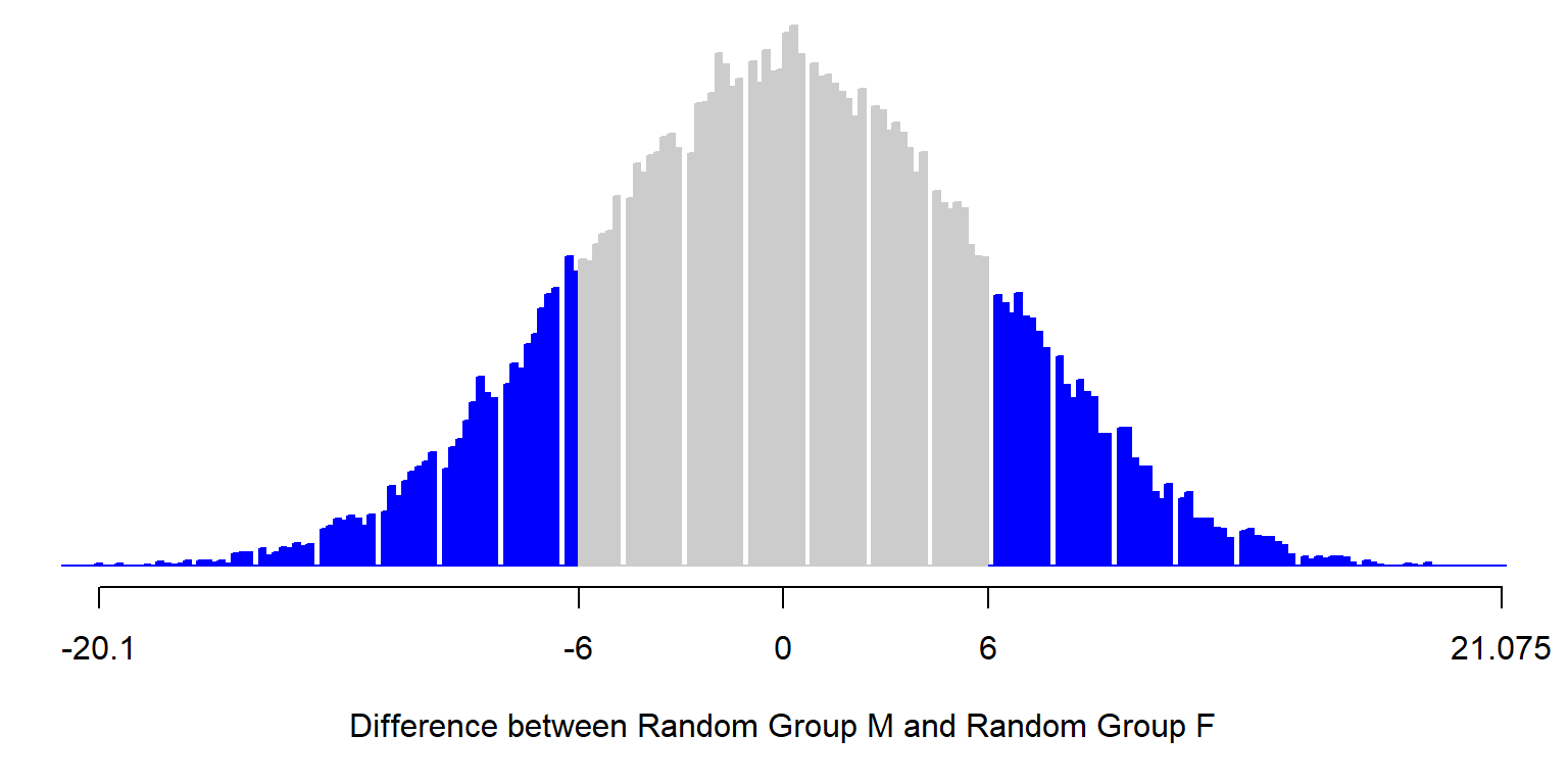
The p-value of 0.31 indicates the strength of evidence that the analysis provided against the null hypothesis that the mean weight of female ISU students equals the mean weight of male ISU students. In particular, the p-value of p=0.31 indicates that, if we randomly assigned students in our sample to a group of 10 and a group of 8, about 31 percent of the time would we expect the difference between these random groups to be at least as large as the 6-pound difference that we observed between the sample of 10 female students and the sample of 8 male students.
The smaller this p-value percentage, the less likely it is that the observed outcome or a more extreme outcome would have occurred if the null hypothesis were true. Therefore, the smaller this p-value percentage, the less likely it is that the null hypothesis is true.
There is a good reason why the p-value calculation involves the percentage of outcomes that are at least as extreme as the observed outcome, instead of the percentage of simulated outcomes that are exactly as extreme as the observed outcome. For an example of eight coin flips, if we counted the percentage of potential outcomes that are exactly as extreme as the observed outcome, then the p-value for four heads in eight flips would be p=0.27, which suggests that the observed outcome provided a good amount of evidence against the null hypothesis that the coin is fair, even though the coin landed on heads 50% of the time and on tails 50% of the time. If instead we count the percentage of potential outcomes that are at least as as extreme as the observed outcome, then the p-value for four heads in eight flips would be p=1, which correctly indicates that the observed outcome provided no evidence against the null hypothesis that the coin is fair.
3.4 p-values if the null hypothesis is true
Suppose that we conduct a large number of tests of a null hypothesis that is true. Below is a plot of the expected distribution of p-values, if the null hypothesis is true. In particular, for this plot, I had the computer randomly draw 200 whole numbers from 0 through 100 and call those 200 numbers X, then randomly draw another 200 whole numbers from 0 through 100 and call those 200 numbers Y, and then test the null hypothesis that the mean of X equals the mean of Y. The computer did that 100,000 times and then plotted the 100,000 p-values in the histogram below. The distribution of p-values when the null hypothesis is true is expected to be a uniform distribution, so that, for example, 5% of p-values are equal to or lower than p=0.05, 20% of p-values are are equal to or lower than p=0.20, 75% of p-values are are equal to or lower than p=0.75, and 100% of p-values are are equal to or lower than p=1.00.
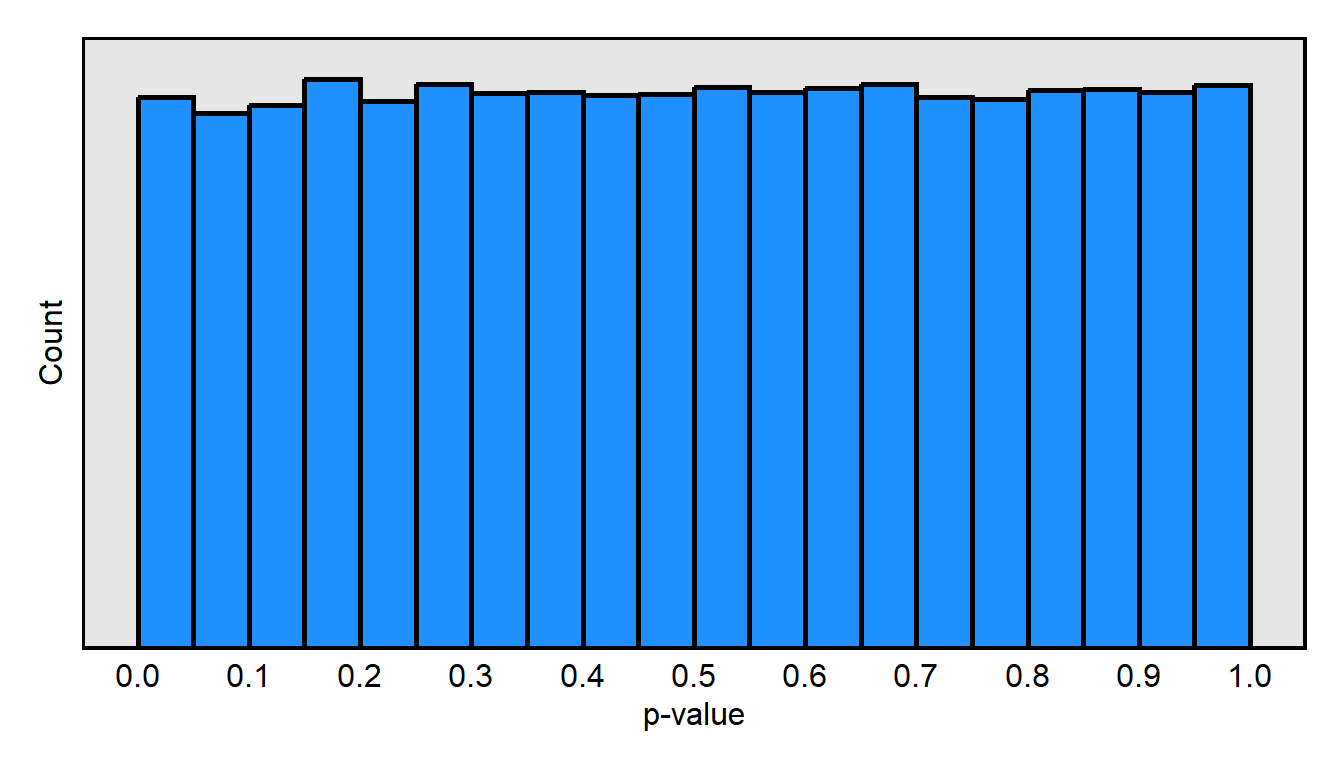
Here is what is going on conceptually, when the null hypothesis is true and, in this case, we are drawing two random samples from the same population. Sometimes – due to random chance – the mean of the first random sample exactly equals the mean of the second random sample, so that the p-value for a test of the null hypothesis is p=1. But sometimes – due to random chance – the mean of the first random sample does not exactly equal the mean of the second random sample, and the p-value for a test of the null hypothesis is p=0.50 or p=0.40 or p=0.90 or any other p-value. And sometimes the mean of the first random sample is so different from the mean of the second random sample that the p-value for a test of the null hypothesis is less than p=0.05, so that we incorrectly reject the null hypothesis. In this case, when the null hypothesis is true, the p-value that we get is a random number between 0 and 1.
Sample practice items
Suppose that we test a null hypothesis that is true. What percentage of the time is the p-value expected to be p<0.05?
- 0% of the time
- about 5% of the time
- about 50% of the time
- about 95% of the time
- 100% of the time
- Cannot be determined without additional information
Answer
- about 5% of the time
3.5 p-values if the null hypothesis is not true
Below is another plot of the distribution of p-values from simulations. The dark gray background indicates the distribution of p-values that is expected to occur if the null hypothesis is true.
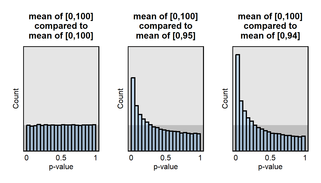
For the left plot, for 100,000 trials, I randomly drew 200 whole numbers from the population [0,100] and 200 whole numbers from the population [0,100] and tested the true null hypothesis that the mean of the first population equaled the mean of the second population. In this simulation, the null hypothesis is true, so the distribution of these p-values is uniform.
For the middle plot, for 100,000 trials, I randomly drew 200 whole numbers from the population [0,100] and 200 whole numbers from the population [0,95] and tested the false null hypothesis that the mean of the first population equaled the mean of the second population. In this simulation, the null hypothesis is not true, so the distribution of these p-values is not uniform, with more p-values under p<0.05 than would be expected if the null hypothesis were true.
For the right plot, for 100,000 trials, I randomly drew 200 whole numbers from the population [0,100] and 200 whole numbers from the population [0,94] and tested the false null hypothesis that the mean of the first population equaled the mean of the second population. In this simulation, the null hypothesis is not true, so the distribution of these p-values is not uniform, with a higher percentage of low p-values relative to the prior comparison, of [0,100] to [0,95].
Here is what is going on conceptually, when the null hypothesis is NOT true and, in this case, we are drawing two random samples from different populations. Sometimes – due to random chance – the mean of the first random sample exactly equals the mean of the second random sample, so that the p-value for a test of the null hypothesis is p=1. But that is expected to happen LESS often when we are randomly sampling from different populations, compared to when we are randomly sampling from the same population. And sometimes – due to random chance – the mean of the first random sample is so different from the mean of the second random sample that the p-value for a test of the null hypothesis is less than p=0.05 so that we incorrectly reject the null hypothesis. But this is expected to happen MORE often when we are randomly sampling from different populations, compared to when we are randomly sampling from the same population.
In this case, when the null hypothesis is NOT true, the p-value that we get is NOT a random number between 0 and 1. Instead, the p-value is more likely to be lower than to be higher.
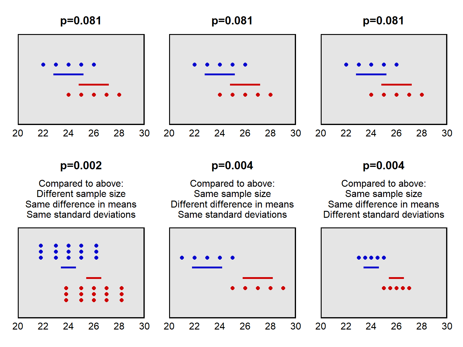
If the null hypothesis is not true, then the size of a p-value can be affected by sample size: all else equal, larger samples provide more evidence, so – if the null hypothesis is not true – larger samples are expected to associate with more evidence against the null hypothesis and thus to associate with smaller p-values, all else equal. The size of a p-value can also be affected by the size of the association: all else equal, larger associations are easier to detect, so – if the null hypothesis is not true – larger associations are expected to associate with smaller p-values, all else equal. And the size of a p-value can be affected by the standard deviation of measurements: the less variation in the measurements, the more certainty we have about the center of the measurements, so – if the null hypothesis is not true – smaller standard deviations are expected to associate with smaller p-values, all else equal.
The plots below illustrate these factors. Imagine that we draw a random sample from Population A (blue) and draw a random sample from Population B (red). In each panel in the plot below, the sample from Population A is plotted higher than the sample from Population B. For each panel in the plot below, we conduct a test of the null hypothesis that the mean of Population A equals the mean of Population B. For the top row of panels, the p-value for a test of this null hypothesis is p=0.08. The horizontal lines in the plot indicate the 83.4% confidence intervals for each set of points. The panel on the bottom left indicates what happens when the sample size is larger. The panel in the bottom middle indicates what happens when the means of the samples are farther apart. The panel in the bottom right indicates what happens when the standard deviation of the points is smaller.
Sample practice items
Suppose that Coin A is flipped 10 times lands on heads 10 times and on tails 0 times. Coin B is flipped 10 times lands on heads 7 times and on tails 3 times. You conduct a statistical test of the null hypothesis that Coin A is fair, and you conduct a statistical test of the null hypothesis that Coin B is fair. For which coin would the p-value from these tests be lower?
- Coin A
- Coin B
- Neither: The p-value for Coin A would be the same as the p-value for Coin B.
Answer
- Coin A
The 10 coin flips of Coin A provided stronger evidence against the null hypothesis that Coin A is fair than the 10 flips of Coin B provided against the null hypothesis that Coin B is fair.
Suppose that Coin A is flipped 10 times lands on heads 10 times and on tails 0 times. Coin B is flipped 100 times lands on heads 100 times and on tails 0 times. You conduct a statistical test of the null hypothesis that Coin A is fair, and you conduct a statistical test of the null hypothesis that Coin B is fair. For which coin would the p-value from these tests be lower?
- Coin A
- Coin B
- Neither: The p-value for Coin A would be the same as the p-value for Coin B.
Answer
- Coin B
The 100 coin flips of Coin B provided stronger evidence against the null hypothesis that Coin B is fair than the 10 flips of Coin A provided against the null hypothesis that Coin A is fair.
Suppose that Coin A is flipped 10 times lands on heads 5 times and on tails 5 times. Coin B is flipped 100 times lands on heads 50 times and on tails 50 times. You conduct a statistical test of the null hypothesis that Coin A is fair, and you conduct a statistical test of the null hypothesis that Coin B is fair. For which coin would the p-value from these tests be lower?
- Coin A
- Coin B
- Neither: The p-value for Coin A would be the same as the p-value for Coin B.
Answer
- Neither: The p-value for Coin A would be the same as the p-value for Coin B.
In both cases, the coin flips provided no evidence against the null hypothesis that the coin is fair.
Suppose that the p-value is p=0.60 for a test of the null hypothesis that the mean of an outcome variable for Group A equals the mean of that outcome variable for Group B, using an outcome variable that is coded from 0 through 100. If we divided the outcome variable by 5, so that the outcome variable is now coded to range from 0 through 20, which of the following, if any, would we know about the p-value for a test of the null hypothesis that the mean of the outcome variable for Group A equals the mean of that outcome variable for Group B?
- The p-value would certainly be p=0.60.
- The p-value would certainly be less than p=0.60.
- The p-value would certainly be greater than p=0.60.
- None of the above
Answer
- The p-value would certainly be p=0.60.
A p-value is a measure of evidence. Dividing the outcome by 5 shouldn’t change the amount of evidence that the analysis provided.
Suppose that Amy has hard copy surveys from 1,000 participants in an experiment. Amy calculated that the p-value was 0.02 for the mean difference in responses between the control group and the treatment group; that mean difference was 3. Amy lost a random half of her hard copy surveys, and she recalculated the p-value for the control/treatment difference in means, based on the 500 hard copy surveys that she still had. Which would be most likely about this new difference in means?
- This difference in means is still about 3.
- This difference in means is lower than 3.
- This difference in means is greater than 3.
Answer
- This difference in means is still about 3.
Randomly losing data would not bias the estimated difference in means, because the data loss was random.
Suppose that Amy has hard copy surveys from 1,000 participants in an experiment. Amy calculated that the p-value was 0.02 for the mean difference in responses between the control group and the treatment group; that mean difference was 3. Amy lost a random half of her hard copy surveys, and she recalculated the p-value for the control/treatment difference in means, based on the 500 hard copy surveys that she still had. Which would be most likely about this new p-value?
- This p-value is still 0.02.
- This p-value is lower than 0.02.
- This p-value is higher than 0.02.
Answer
- This p-value is higher than 0.02.
Randomly losing data means that you have less evidence, so the p-value likely will get closer to 1 (because 1 means no evidence against the null hypothesis).
Suppose that Amy and Bob each have a class of five students, each of whom takes a pretest and a posttest. The pretest-to-posttest changes in scores for Amy’s students are: +1, +4, +3, +5, and +2, so that the mean change among Amy’s students is +3. The pretest-to-posttest changes in scores for Bob’s students are: +7, -4, -2, -3, and +17, so that the mean change among Bob’s students is +3. Amy calculates a p-value for a test of the null hypothesis that the mean change among Amy’s students is zero; that p-value is p=0.013. What should be expected about the p-value for a test of the null hypothesis that the mean change among Bob’s students is zero?
- That p-value is also p=0.013.
- That p-value is under p=0.013.
- That p-value is above p=0.013.
Answer
- That p-value is above p=0.013.
All else equal, larger standard deviations produce more uncertainty about the mean of data, so Bob’s p-value will be above p=0.013.
Suppose that we test a null hypothesis that is true. What percentage of the time is the p-value expected to be p<0.05?
- 0% of the time
- about 5% of the time
- about 50% of the time
- about 95% of the time
- 100% of the time
- Cannot be determined without additional information
Answer
- about 5% of the time
Suppose that we test a null hypothesis that is NOT true. What percentage of the time is the p-value expected to be p<0.05?
- 0% of the time
- about 5% of the time
- about 50% of the time
- about 95% of the time
- 100% of the time
- Cannot be determined without additional information
Answer
- Cannot be determined without additional information
3.6 Hypothesis testing
A p-value indicates the strength of evidence that an analysis has provided against the null hypothesis. Researchers can merely report the p-value for an analysis, but researchers can also use the p-value in a hypothesis test to make a decision, such as whether to consider that the analysis has provided sufficient evidence against the null hypothesis.
The process for a hypothesis test is to:
- Select a null hypothesis.
- Select a p-value threshold that indicates what will be considered sufficient evidence against the null hypothesis.
- Conduct an analysis to test the null hypothesis.
- Calculate a p-value that indicates the amount of evidence that the analysis has provided against the null hypothesis.
- If the calculated p-value is less than the p-value threshold, then reject the null hypothesis and accept the alternative hypothesis; otherwise, do not accept and do not reject the null hypothesis or the alternative hypothesis.
In political science, the conventional threshold for rejecting the null hypothesis is a p-value of p=0.05, such that we reject the null hypothesis and accept the alternative hypothesis if and only if the p-value is less than p=0.05. To provide a sense of the amount of evidence that this p=0.05 threshold represents, for a test of the null hypothesis that a coin is fair, the p-value would be about 0.06 if the coin landed on heads 5 times in 5 flips.
Suppose that our null hypothesis is that a coin is fair. We flip the coin 20 times and get 15 heads and 5 tails. The p-value for this would be p=0.041. This p-value is less than 0.05, so we reject the null hypothesis that the coin is fair; and, given that the we reject the null hypothesis that the coin is fair, we can accept the alternative hypothesis that the coin is unfair.
But suppose that our null hypothesis is that a coin is fair, and we flip the coin 2 times and get 2 heads and 0 tails. The p-value would be p=0.50. This p-value is not less than 0.05, so we do not reject the null hypothesis that the coin is fair. But we also don’t accept the null hypothesis that the coin is fair: each time we flipped the coin, the coin landed on heads, so we don’t want to accept the hypothesis that the coin is fair. In this case, we merely decline to conclude anything about the null hypothesis.
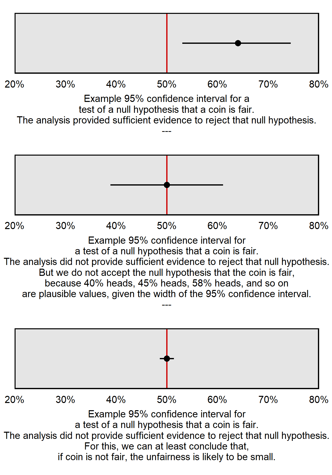
Let’s use the plot below to illustrate why the null hypothesis is never accepted. Each of the three panels is a 95% confidence interval for a different set of flips of a different coin. For each coin flip, let’s test the null hypothesis that the coin is fair. The 95% confidence interval in the top panel does not include the 50% heads that we expect in the long run from a fair coin, so we can reject the null hypothesis that the coin is fair. The middle panel and the bottom panel each have 95% confidence intervals that include the 50% heads that we expect in the long run from a fair coin, so we cannot reject the null hypothesis that the coin is fair for the middle panel or the bottom panel. But check the width of the 95% confidence interval for the middle panel, which extends from 39% heads to 61% heads: a 95% confidence interval contains the range of plausible values based on our analysis, so – based on our analysis – it’s plausible that the coin could be unfair and truly have an 11 percentage point bias toward heads, an 11 percentage point bias toward tails, or a smaller bias in between. So, in the middle panel, while we can’t use the 95% confidence interval to reject the null hypothesis that coin is fair, we also can’t use the 95% confidence interval to accept the null hypothesis and conclude that the coin is fair. The explanation is similar for the 95% confidence interval in the bottom panel, which extends from 49% heads to 51% heads. However, the range of the 95% confidence interval in the bottom panel is so tight around 50% heads that we can conclude that, if the coin is not fair, the unfairness of the coin is likely to be relatively small, at no more than 1 percentage point toward heads or no more than 1 percentage point toward tails.
For the type of statistics that we practice in this course, we never accept the null hypothesis. For another illustration why, suppose that we flip a coin 2 times and get 1 head and 1 tail. The p-value will be 1, which indicates that the analysis provided no evidence against the null hypothesis. But we should not accept the null hypothesis because we flipped the coin only two times, and those two flips don’t provide much information about whether the coin is fair.
But even though we never accept the null hypothesis, we can use 95% confidence intervals to infer that, if the null hypothesis is not true, then the null hypothesis is pretty close to true. For example, if we flip a coin 10,000 times and get 5,000 heads and 5,000 tails, the 95% confidence interval for the percentage heads will be [49%, 51%], so, in that case, we can conclude that, if the coin is not fair, then the unfairness of the coin is likely very small.
Sample practice items
What is the conventional p-value threshold in political science?
- 0
- 0.01
- 0.05
- 0.50
- 0.95
- 1
Answer
- 0.05
Given the conventional threshold for rejecting the null hypothesis in political science, if the p-value is p=0.01 for the test of a null hypothesis, then which, if any, of the following should we do?
- Accept the null hypothesis and the alternative hypothesis.
- Reject the null hypothesis and the alternative hypothesis
- Accept the null hypothesis, but reject the alternative hypothesis.
- Reject the null hypothesis, but accept the alternative hypothesis.
- None of the above
Answer
- Reject the null hypothesis, but accept the alternative hypothesis.
The p-value is lower than p=0.05, so we can reject the null hypothesis that the coin is fair and accept the alternative hypothesis that the coin is unfair.
Given the conventional threshold for rejecting the null hypothesis in political science, if the p-value is p=0.49 for the test of a null hypothesis, then which, if any, of the following should we do?
- Accept the null hypothesis and the alternative hypothesis.
- Reject the null hypothesis and the alternative hypothesis
- Accept the null hypothesis, but reject the alternative hypothesis.
- Reject the null hypothesis, but accept the alternative hypothesis.
- None of the above
Answer
- None of the above
The p-value is not lower than p=0.05, so we do not accept or reject either the hypothesis.
3.7 Selecting a p-value threshold
The conventional p-value threshold in political science is p=0.05. This p-value threshold of p=0.05 means that, if the null hypothesis is true, we will have a 5% chance of incorrectly rejecting the null hypothesis.
But sometimes a different p-value threshold is more appropriate. For instance, if we want to better avoid a false positive in which we incorrectly reject a true null hypothesis, then we can lower the p-value to something such as p=0.01 or p=0.001, so that we require more evidence to reject the null hypothesis. Or, if we want to better avoid a false negative in which we incorrectly do not reject a false null hypothesis, then we can raise the p-value to something such as p=0.10, so that we require less evidence to reject the null hypothesis.
| p-value threshold | What the p-value threshold requires in order to reject the null hypothesis |
|---|---|
| 1 | Requires no evidence against the null hypothesis |
| 0.99 | Requires a very small amount of evidence against the null hypothesis |
| 0.98 | Requires a bit more evidence against the null hypothesis |
| … | … |
| 0.01 | Requires a lot of evidence against the null hypothesis |
| 0 | Requires infinitely strong evidence against the null hypothesis |
The conventional p-value threshold in political science is p=0.05. Having a conventional threshold is useful for shorthand communication about whether an analysis has provided enough evidence against the null hypothesis, but we should not invest too much importance in that p=0.05 threshold: the amount of evidence reflected in a p-value of p=0.051 is pretty close to the amount of evidence reflected in a p-value of p=0.049, even though only the second p-value permits us to claim sufficient evidence against the null hypothesis at the conventional level in political science.
Sample practice items
Suppose that we test athlete DNA samples for evidence of their use illegal performance-enhancing substances. The null hypothesis is that the athlete is not using illegal performance-enhancing substances. Which p-value threshold below would be more appropriate if we wanted to better avoid a false conclusion that an athlete is using steroids?
- p=0.01
- p=0.10
Answer
- p=0.01
Compared to a p-value threshold of p=0.10, requiring the p-value to be under the p=0.01 threshold means that there will be more evidence that the athlete is using illegal performance-enhancing substances.
Researchers are testing athlete urine samples for illegal substances. The researchers will test any sample that tests positive on the first test at least three more times after an initial positive test before the athlete is suspended for use of illegal substances, so – for the first test of the samples – the researchers would much rather erroneously conclude that a sample contains illegal substances than to erroneously conclude that the sample does not contain illegal substances. Which p-value threshold below would be more appropriate, for this first test of the null hypothesis that the urine samples does not contain an illegal substance?
- p=0.01
- p=0.10
Answer
- p=0.10
The conventional threshold for accepting a political science association as indicating a true association is a p-value under 0.05. If we want to have fewer false positives in which we falsely reject the null hypothesis, which of the following could we do?
- lower the p-value threshold to 0.01
- raise the p-value threshold to 0.10
Answer
- lower the p-value threshold to 0.01
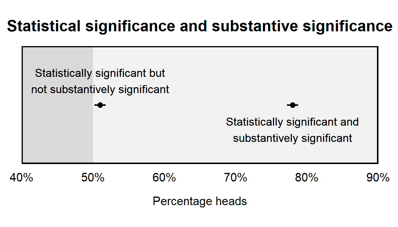
3.8 Statistical and substantive significance
Research sometimes refers to a “statistically significant” result, which is shorthand for a result for which an analysis has provided sufficient evidence against the null hypothesis. If the null hypothesis is that there is no association, then “statistically significant” evidence provided evidence evidence that the association exists, but the phrase “statistically significant evidence” does not indicate whether this association is large or important or causal. Research can make a distinction between “statistical significance” and “substantive significance”; this “substantive significance” refers to whether the estimated effect is large enough to be important.
This distinction between statistical significance and substantive significance is important, because an analysis might indicate statistical significance without indicating substantive significance. That’s because, even if the effect is substantively small, it’s possible to get a p-value indicating a lot of evidence against the null hypothesis. For instance, if a coin flipped 1 million times landed on heads 50.2% of time, the coin isn’t very unfair, but the associated p-value would be very small, at p=0.000064. In this example, the unfairness of the coin is very small, but we have a lot of evidence that this unfairness exists.
Similarly, if an effect is large, it’s possible to get a p-value indicating relatively little evidence against the null hypothesis. For instance, suppose that we have a two-headed coin. If this coin is flipped 2 times and landed on heads 100% of time, the p-value would be p=0.50 for a test of the null hypothesis that the coin is fair. In this example, the unfairness of the coin is large (never landing on tails), but we have relatively little evidence that this unfairness exists.
Here is an example of a “statistically significant” result for an effect that is relatively small in substantive terms, from Wen and Burke 2022:
Relative to a school year with no smoke, average cumulative smoke-attributable PM2.5 (surface particulate matter <2.5 μg m−3) exposure during the school year (~35 μg m−3) reduces test scores by ~0.15% of a standard deviation.
So how big is 0.15% of a standard deviation? Let’s use heights as an analogy. Based on Our World in Data, the standard deviation of male heights in North America is 7.49 cm, which is about 3 inches, and 0.15% of 3 inches is 0.0045 inches.
Sample practice items
For a test of the null hypothesis that there is no association, the term “statistically significant evidence” refers to…
- sufficient evidence that the association is large
- sufficient evidence that the association exists
Answer
- sufficient evidence that a particular association exists
If the p-value is p=0.0000001 for a single statistical test of a null hypothesis that there is no association, do we have enough evidence to claim that there is statistically significant evidence for the detected association?
- Yes
- No
Answer
- Yes
Suppose that the p-value is p=0.0000001 for a test that a coin is fair. Based on this, can we conclude that the coin is very unfair?
- Yes
- No
Answer
- No
For a test of the null hypothesis that a coin is fair, a p-value indicates the strength of evidence against that hypothesis. The p-value by itself does not indicate anything about how unfair the coin might be. A low p-value can be caused by a slightly unfair coin flipped a large number of times, a very unfair coin flipped a smaller number of times, or other combinations of unfairness and number of coin flips. All the small p-value indicates is that the analysis provided a lot of evidence that the coin is unfair.
3.9 Hypothesis tests involving random sampling
If a sample is a random sample of a population, the only difference between the characteristics of the sample and the characteristics of the population will be due to random chance, such as if, by random chance, the sample had too many females or too many males or too many Democrats or too many Republicans, relative to the population. For example, if a population has 500 males and 500 females, a random sample of that population is expected to be about 50% female, but – due to random chance – the random sample might sometimes have 46% females or 52% females or 55% females or any other percentage of females.
This difference between the characteristics of a random sample and the characteristics of the population is random sampling error. We can’t avoid random sampling error, but we can use a p-value to assess the plausibility that our sample is not representative of the population. In particular, a p-value of p<0.05 permits us to eliminate random sampling error as a plausible alternate explanation.
Note that the discussion in this subsection refers to random samples of a population, which are plausibly representative of the population. If the sample is plausibly different from the population in a relevant way, then the p-value is irrelevant. For example, if we randomly sample 500 Illinois Democrats, then that sample plausibly isn’t representative of the population of Illinois residents, so any political measure drawn from that sample will likely be biased, so that any p-value is useless for helping to make inferences about the population.
3.10 Caution about p-values for causal inference
p-values and hypothesis tests are useful for making descriptive inferences, such as whether two variables associate with each other or whether the mean of one population differs from the mean of another population. For example, we can randomly sample 100 people who graduated from college, randomly sample 100 people who did not graduate from college, and then calculate a p-value to test the null hypothesis that the mean income among people who graduated from college equals the mean income among people who did not graduate from college. If the p-value for that test is p<0.05, then we have sufficient evidence at the conventional level in political science that these mean incomes differ from each other. But that p-value of p<0.05 by itself does not let us infer that graduating from college caused these mean incomes to differ from each other. To make such a causal inference, we would need to consider other potential explanations for the observed difference. For example, maybe people who graduate from college are on average more intelligent than people who do not graduate from college, and maybe this possible on-average difference in intelligence is the reason for the difference in mean incomes between these groups. Our analysis should address this potential explanation before we make an inference that college caused the observed on-average difference in mean income.
Sample practice items
Suppose that a police department has 2,000 police officers. The department received a shipment of 400 body cams and solicited volunteers to wear a body camera for the next three months. Results indicated that the mean number of citizen complaints was lower among the police officers who volunteered to wear a body camera than among the police officers who did not wear a body camera, with a p-value of p<0.05 for a test of the null hypothesis that these means equaled each other. Is that sufficient evidence at the conventional level in political science that wearing a body camera caused a lower number of citizen complaints, on average, among this police department?
- Yes
- No
Answer
- No
There are alternate explanations that should be addressed before concluding causality. For example, maybe the police officers who volunteered to wear a body camera received a fewer number of complaints than other officers, even before wearing the body camera. These police officers who chose to wear a body camera thus might have been better behaved, older, or have some other characteristic that caused the lower number of citizen complaints.
3.11 One-tailed p-values
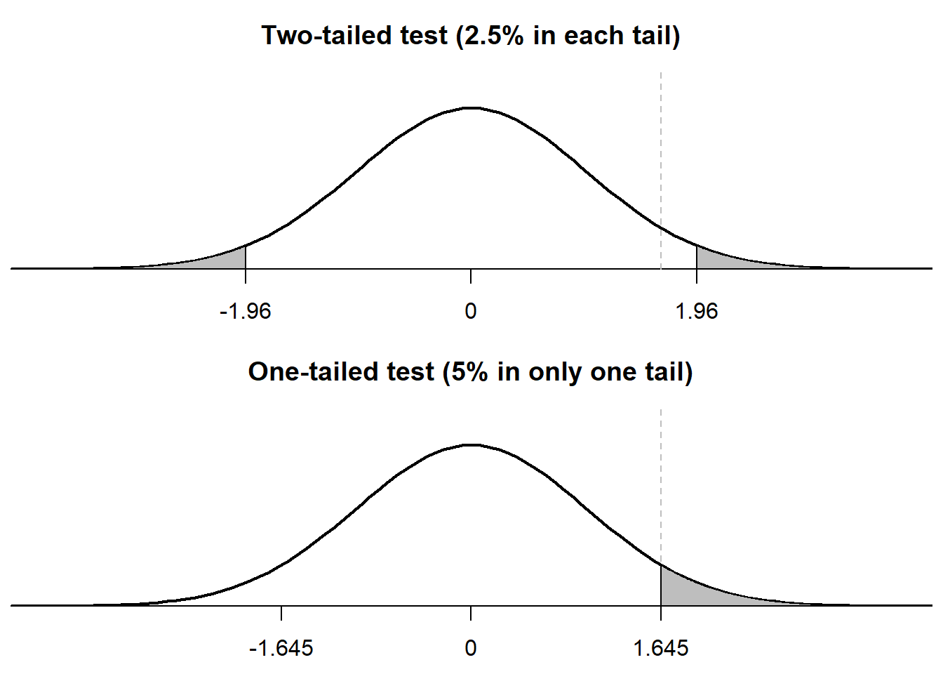
The p-values that we have discussed so far are p-values from a two-tailed test (aka a two-sided test). A two-tailed test permits us to detect associations in both directions: for example, with a two-tailed test, we could detect a coin that lands on heads more often than tails, and we can detect a coin that lands on tails more often than heads. But sometimes some researchers use a one-tailed test that permits us to detect associations in only one direction, so that we could detect that the coin lands on heads more than tails but we could not detect that the coin lands on tails more than heads. Hopefully, a test that can detect associations in only one direction should seem like a bad idea to you. We will avoid conducting one-tailed tests in this course.
An important feature of a one-tailed test is that, compared to a two-tailed test, a one-tailed test requires less evidence to reject a null hypothesis, as indicated in the plots below. The top plot illustrates how, for a p-value of p=0.05, the two-tailed test assigns 0.025 to the left tail and assigns 0.025 to the right tail, and the two-tailed test rejects the null hypothesis if and only if the observed association is in the gray region. The bottom plot illustrates how, for a p-value of p=0.05, the one-tailed test assigns 0.05 to only one of the tails, and the one-tailed test rejects the null hypothesis if and only if the observed association is in the gray region. But for the one-tailed test, the gray region is closer to zero and thus requires less evidence, provided that the association is in the hypothesized direction.