10 Limited outcome variables
10.1 Dichotomous outcome variables
For an OLS linear regression, the statistical program draws a straight line of best fit through the data points. The coefficients for predictors in an OLS linear regression indicate the slope of a line, so the coefficients can be interpreted as the change in the outcome predicted for a one-unit change in the predictor, holding other predictors constant. But other types of regression predict an outcome using curves instead of a straight line, so that the interpretation of the coefficients can’t be made as if the coefficient were the slope of a straight line, because a curve does not have a single slope.
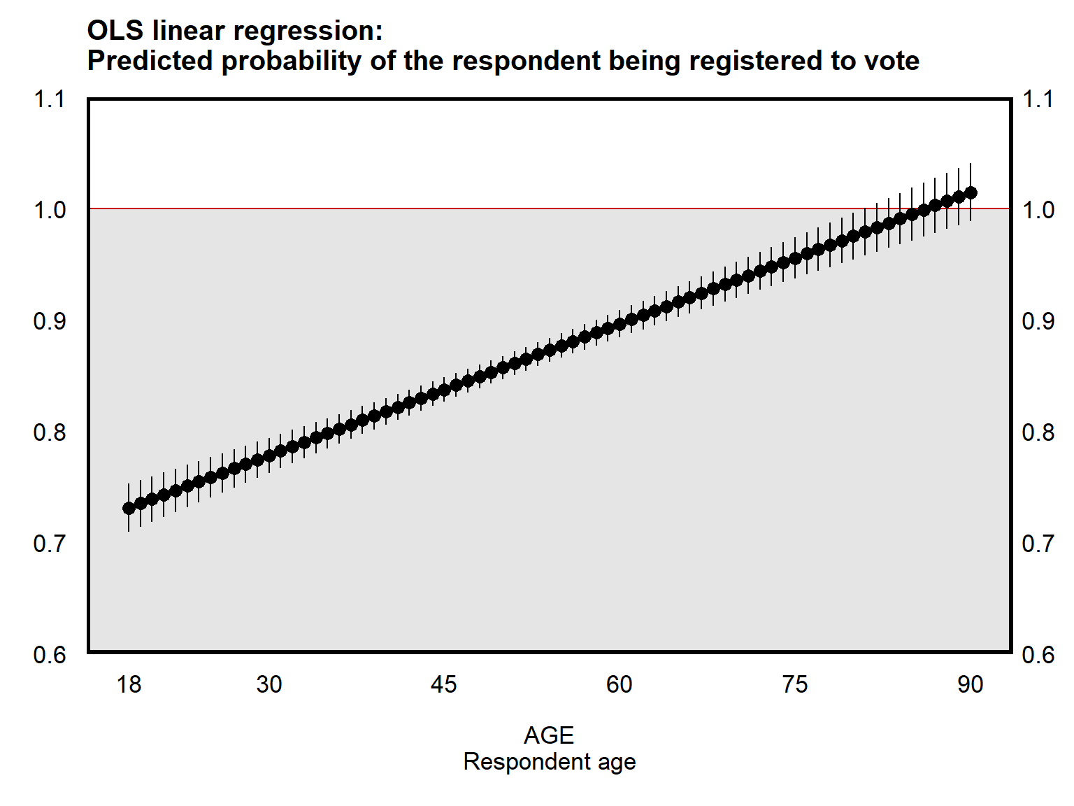
Below is a plot from an OLS linear regression based on data from the ANES 2016 Time Series Study. The plot uses respondent age to predict the probability that the respondent reported being registered to vote. The outcome variable measured whether the respondent reported being registered to vote, coded 0 for respondents who did not indicate that they registered to vote or indicated that they were not registered to vote, and coded 1 for respondents who reported being registered to vote. This type of outcome can be referred to as a binary or dichotomous outcome, in which the outcome takes on only two possible values (coded 0 and 1). The line of best fit for a dichotomous outcome variable can be thought of the predicted probability that the outcome is 1, in which 0 is a 0% predicted probability that the outcome is 1, 0.5 is a 50% predicted probability that the outcome is 1, and 1 is a 100% predicted probability that the outcome is 1.
The plot below used a linear regression to get estimates of the predicted probability that the respondent reported being registered to vote. This is called the linear probability model, because the model predicts probabilities using a linear regression. One shortcoming of the linear probability model is that the linear probability model can produce predictions that are impossible, such as a 90-year-old respondent respondent having a predicted probability of being registered to vote that is greater than 100%.
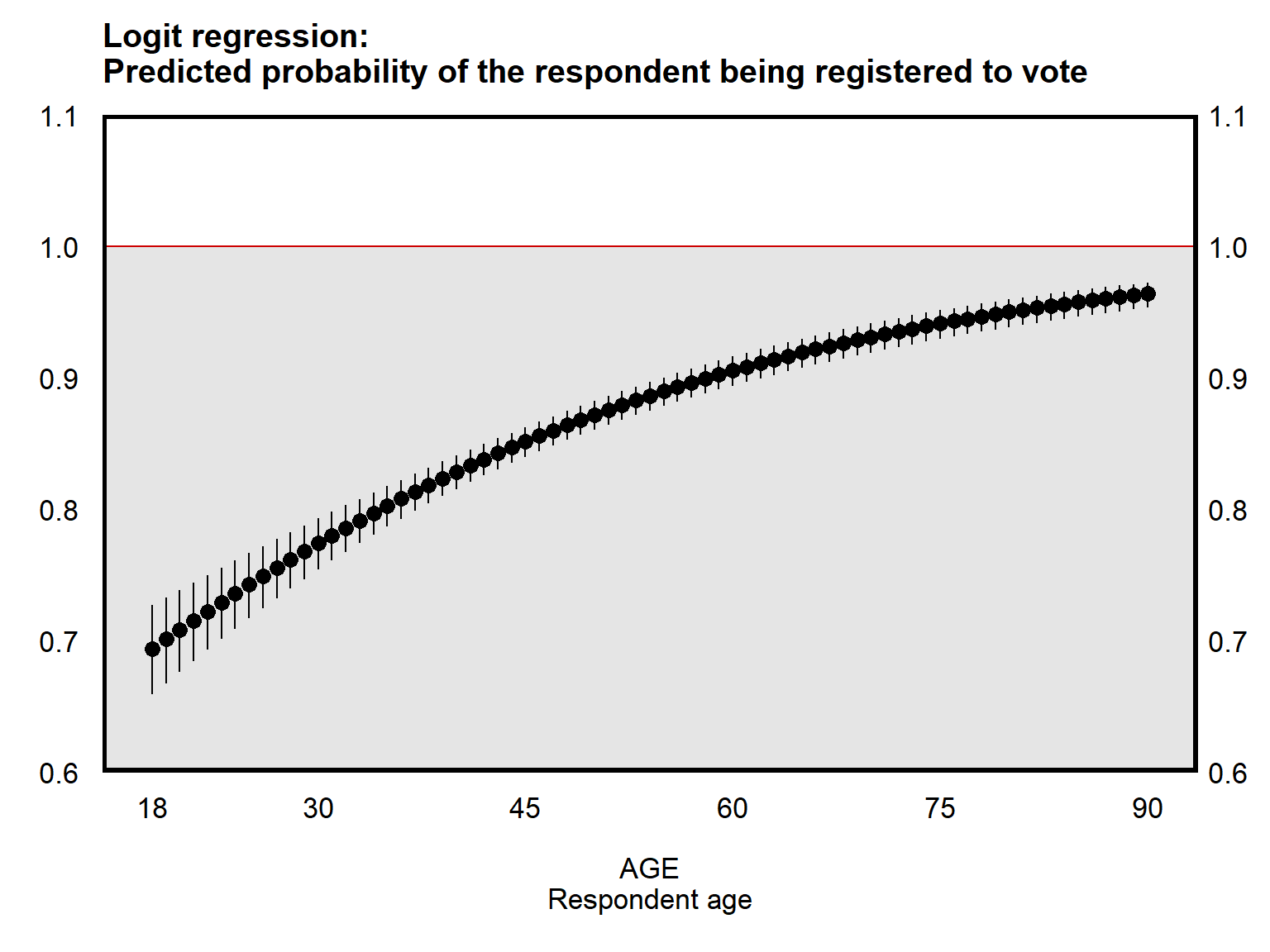
Below is a plot of the same data, but using an estimation technique called a logistic regression, in which all predictions are restricted to fall within the range of 0 to 1. The tradeoff for a “logit” regression is that the line of best fit is not a straight line, so the logit regression output is more difficult to interpret.
Below is output for the linear probability model. The output indicates that the REGISTERED outcome is predicted to increase by 0.0039 units for each one-unit increase in the AGE predictor. The REGISTERED outcome is coded 0 or 1, so the 0.0039 coefficient on the AGE predictor can be interpreted as a probability: compared to the probability that a participant at a given age reported being registered to vote, the probability that a participant one year older than that reported being registered to vote is predicted to be 0.39 percentage points higher.
reg REGISTERED AGE, noheader
running D:\OneDrive - IL State University\2-teaching\R for teaching\POL497\prof

> ile.do ...


------------------------------------------------------------------------------
  REGISTERED |      Coef.   Std. Err.      t    P>|t|     [95% Conf. Interval]
-------------+----------------------------------------------------------------
         AGE |     0.0039     0.0003    12.94   0.000       0.0033      0.0045
       _cons |     0.6603     0.0160    41.23   0.000       0.6289      0.6917
------------------------------------------------------------------------------
Let’s check the logit regression output:
logit REGISTERED AGE, noheader nolog
running D:\OneDrive - IL State University\2-teaching\R for teaching\POL497\prof

> ile.do ...


------------------------------------------------------------------------------
  REGISTERED |      Coef.   Std. Err.      z    P>|z|     [95% Conf. Interval]
-------------+----------------------------------------------------------------
         AGE |     0.0343     0.0028    12.34   0.000       0.0289      0.0398
       _cons |     0.2015     0.1266     1.59   0.111      -0.0466      0.4496
------------------------------------------------------------------------------
The logit coefficient of 0.0343 for the AGE predictor is not a slope, because the logit predictions fall on a curve and not on a straight line. The 0.0343 coefficient is instead an estimate of the change in the log of the odds ratio for the outcome, based on a one-unit change in the predictor, net of controls. The interpretation for a logit coefficient is relatively complicated to explain (and to understand), so it’s likely easier for readers if you plot logit results or if you report predicted probabilities for a logit regression, like in the plot above, than to merely report logit coefficients in a table.
The “nolog” option omits output about iterations used to fit the model. We typically don’t need that output, but let’s see that output below:
logit REGISTERED AGE, noheader
running D:\OneDrive - IL State University\2-teaching\R for teaching\POL497\prof

> ile.do ...


Iteration 0:   log likelihood = -1712.7963
Iteration 1:   log likelihood = -1632.4084
Iteration 2:   log likelihood = -1629.0562
Iteration 3:   log likelihood = -1629.0468
Iteration 4:   log likelihood = -1629.0468
------------------------------------------------------------------------------
  REGISTERED |      Coef.   Std. Err.      z    P>|z|     [95% Conf. Interval]
-------------+----------------------------------------------------------------
         AGE |     0.0343     0.0028    12.34   0.000       0.0289      0.0398
       _cons |     0.2015     0.1266     1.59   0.111      -0.0466      0.4496
------------------------------------------------------------------------------
Sample practice items
The output below is from a logit regression using respondent AGE (coded from 18 to 80) to predict VOTETC, which is a measure of whether the respondent reported voting for Donald Trump (coded 1) or Hillary Clinton (coded 0) in the 2016 U.S. presidential election. The data are from the ANES 2016 Time Series Study.
logit VOTETC AGE, noheader nolog
running D:\OneDrive - IL State University\2-teaching\R for teaching\POL497\prof

> ile.do ...


------------------------------------------------------------------------------
      VOTETC |      Coef.   Std. Err.      z    P>|z|     [95% Conf. Interval]
-------------+----------------------------------------------------------------
         AGE |      0.015      0.002     6.36   0.000        0.010       0.019
       _cons |     -0.880      0.129    -6.81   0.000       -1.134      -0.627
------------------------------------------------------------------------------
The p-value on AGE is p<0.05. Can this be interpreted to indicate that, among this sample of respondents and on average, a respondent’s age associated with whether the respondent reported voting for Donald Trump or Hillary Clinton in the 2016 U.S. presidential election?
- Yes
- No
Answer
- Yes. Logit p-values can be interpreted as linear regression p-values.
The p-value on AGE is p<0.05, and the coefficient on AGE is 0.015. Can this be interpreted to indicate that, among this sample of respondents and on average, older respondents had a higher probability of reported having voted for Donald Trump instead of Hillary Clinton in the 2016 U.S. presidential election?
- Yes
- No
Answer
- Yes. Logit coefficients can be interpreted as linear regression coefficients in terms of the direction of association with the outcome, net of any other predictors in the regression.
The p-value on AGE is p<0.05, and the coefficient on AGE is 0.015. Can this be interpreted to indicate that, among this sample of respondents and on average, a one-year increase in respondent age associated with a 0.015 increase in the predicted probability that a respondent reported voting for Donald Trump instead of Hillary Clinton in the 2016 U.S. presidential election?
- Yes
- No
Answer
- No. Logit coefficients indicate a change in the log of the odds of the outcome. Logit coefficients cannot be interpreted as linear regression coefficients in terms of substantive size.
10.2 How a logit regression keeps predictions between 0 and 1
Let’s use a simplified formula to explain how a logistic regression keeps predictions between 0 and 1. The p below represents a decimal probability that serves as our outcome:
p = \(\Large\frac{e^X}{1 + e^X}\)
e is a number that is about 2.718.
Let’s plug -10 in for our X predictor, to get
p = \(\Large\frac{2.718^{-10}}{1 + 2.718^{-10}}\)
This equals 0.0000454, which is very close to zero but is slightly above zero.
Let’s plug +10 in for X, to get
p = \(\Large\frac{2.718^{+10}}{1 + 2.718^{+10}}\)
This equals 0.9999546, which is very close to 1 but is slightly below 1.
Any number that you plug in for X will produce a predicted probability that falls between 0 and 1.
Plug in 0 for X, and the predicted probability will be 0.5, representing 50 percent. So if the logit coefficient for a predictor is zero, then that indicates that the predictor does not associate with the probability that the outcome is 1, net of other predictors in the regression. If the logit coefficient is negative, then that indicates that an increase in the predictor associates with a lower probability that the outcome is 1, net of other predictors in the regression. And if the logit coefficient is positive, then that indicates that an increase in the predictor associates with a higher probability that the outcome is 1, net of other predictors in the regression. That interpretation for a logit coefficient – a zero coefficient is no change, a negative coefficient is a negative association, and a positive coefficient is a positive association – matches the interpretation for a linear regression coefficient, although the logit coefficient cannot be interpreted as a slope. Moreover, in a logit regression, the p-values associated with a predictor’s coefficient can also be interpreted as in a linear regression, in these sense of a p-value of p<0.05 providing sufficient evidence that the association is not zero.
10.3 More on logit coefficients
To calculate predicted probabilities by hand, we can treat the logit regression output as a linear regression output, consider the predicted outcome from the linear regression to be X, and then plug that X into the equation:
p = \(\Large\frac{e^X}{1 + e^X}\)
Let’s try that, using the output below, in which a logit regression was used to predict whether a respondent reported being registered to vote, using a predictor of respondent age:
logit REGISTERED AGE, noheader nolog
running D:\OneDrive - IL State University\2-teaching\R for teaching\POL497\prof

> ile.do ...


------------------------------------------------------------------------------
  REGISTERED |      Coef.   Std. Err.      z    P>|z|     [95% Conf. Interval]
-------------+----------------------------------------------------------------
         AGE |   .0343476   .0027824    12.34   0.000     .0288942     .039801
       _cons |   .2015047   .1266043     1.59   0.111    -.0466351    .4496445
------------------------------------------------------------------------------
Let’s get the initial equation, as if this were a linear regression:
REGISTERED = 0.2015047 + 0.0343476*AGE
Let’s start with the predicted outcome for a 20-year-old respondent:
REGISTERED = 0.2015047 + 0.0343476*AGE

REGISTERED = 0.2015047 + 0.0343476*20

REGISTERED = 0.8884567
Now let’s plug that into the logit formula, to get a predicted probability that a typical 20-year-old respondent reported being registered to vote:
p = \(\Large\frac{e^X}{1 + e^X}\) = \(\Large\frac{e^{0.8884567}}{1 + e^{0.8884567}}\) = 0.70857
So the predicted probability that a 20-year-old respondent reported being registered to vote is about 71%. Let’s see what the predicted probability is for a 70-year-old respondent:
REGISTERED = 0.2015047 + 0.0343476*AGE

REGISTERED = 0.2015047 + 0.0343476*70

REGISTERED = 2.6058367
Now let’s plug that into the logit formula, to get a predicted probability that a typical 70-year-old respondent reported being registered to vote:
p = \(\Large\frac{e^X}{1 + e^X}\) = \(\Large\frac{e^{2.6058367}}{1 + e^{2.6058367}}\) = 0.93124
So the predicted probability that a 70-year-old respondent reported being registered to vote is about 93%.
Let’s check the calculations above, using the Stata margins command:
margins, at(AGE=20)
running D:\OneDrive - IL State University\2-teaching\R for teaching\POL497\prof

> ile.do ...


Adjusted predictions                            Number of obs     =      4,149
Model VCE    : OIM

Expression   : Pr(REGISTERED), predict()
at           : AGE             =          20

------------------------------------------------------------------------------
             |            Delta-method
             |     Margin   Std. Err.      z    P>|z|     [95% Conf. Interval]
-------------+----------------------------------------------------------------
       _cons |   .7085716   .0159404    44.45   0.000      .677329    .7398141
------------------------------------------------------------------------------
margins, at(AGE=70)
running D:\OneDrive - IL State University\2-teaching\R for teaching\POL497\prof
> ile.do ...
Adjusted predictions Number of obs = 4,149
Model VCE : OIM
Expression : Pr(REGISTERED), predict()
at : AGE = 70
------------------------------------------------------------------------------
| Delta-method
| Margin Std. Err. z P>|z| [95% Conf. Interval]
-------------+----------------------------------------------------------------
_cons | .9312363 .0056847 163.81 0.000 .9200944 .9423781
------------------------------------------------------------------------------Let’s discuss the “change in the log of the odds ratio” interpretation for a logit coefficient. Below is a logit regression predicting whether a respondent reported being registered to vote, using a predictor for the number of days per week that the respondent consumes news (NEWS, which ranges from 0 to 7):
logit REGISTERED NEWS, noheader nolog
running D:\OneDrive - IL State University\2-teaching\R for teaching\POL497\prof

> ile.do ...


------------------------------------------------------------------------------
  REGISTERED |      Coef.   Std. Err.      z    P>|z|     [95% Conf. Interval]
-------------+----------------------------------------------------------------
        NEWS |   .2698083    .019929    13.54   0.000     .2307481    .3088684
       _cons |   .3950937   .1052549     3.75   0.000     .1887978    .6013895
------------------------------------------------------------------------------
margins, at(NEWS=(0(1)7))
running D:\OneDrive - IL State University\2-teaching\R for teaching\POL497\prof
> ile.do ...
Adjusted predictions Number of obs = 4,266
Model VCE : OIM
Expression : Pr(REGISTERED), predict()
1._at : NEWS = 0
2._at : NEWS = 1
3._at : NEWS = 2
4._at : NEWS = 3
5._at : NEWS = 4
6._at : NEWS = 5
7._at : NEWS = 6
8._at : NEWS = 7
------------------------------------------------------------------------------
| Delta-method
| Margin Std. Err. z P>|z| [95% Conf. Interval]
-------------+----------------------------------------------------------------
_at |
1 | .5975083 .025313 23.60 0.000 .5478958 .6471208
2 | .6603607 .0196537 33.60 0.000 .6218402 .6988811
3 | .7180299 .0144206 49.79 0.000 .689766 .7462938
4 | .7693276 .0101355 75.90 0.000 .7494625 .7891927
5 | .8137141 .0071823 113.30 0.000 .7996372 .8277911
6 | .8512115 .0056957 149.45 0.000 .8400482 .8623748
7 | .8822533 .0052911 166.74 0.000 .871883 .8926236
8 | .9075224 .0052815 171.83 0.000 .8971708 .9178739
------------------------------------------------------------------------------For a respondent who consumes news 0 days per week, the predicted probability of reporting being registered to vote is 0.5975083, so the predicted probability of reporting not being registered to vote for this respondent is 1 minus 0.5975083, which is 0.4024917. The odds that this respondent reported being registered to vote is thus \(0.5975083 \div 0.4024917\), which is 1.484523283.
For a respondent who consumes news 1 day per week, the predicted probability of reporting being registered to vote is 0.6603607, so the predicted probability of reporting not being registered to vote for this respondent is 0.3396393. The odds that this respondent reported being registered to vote is thus \(0.6603607 \div 0.3396393\), which is 1.944300027.
Comparing the first respondent at NEWS=0 to the second respondent at the next higher level of NEWS, the odds ratio is thus \(1.944300027 \div 1.484523283\), which is 1.309713394. And the log of the odds ratio is ln(1.309713394), which is 0.26980833, which is the logit coefficient on the NEWS predictor.
Note that this calculation would work for any one-unit change in NEWS. Let’s check a one-unit change from NEWS=4 to NEWS=5.
For NEWS=5, the predicted probability is 0.8512115, so the odds are: \(\Large\frac{0.8512115}{1 - 0.8512115}\), which is 5.720949536.
For NEWS=4, the predicted probability is 0.8137141, so the odds are: \(\Large\frac{0.8137141}{1 - 0.8137141}\), which is 4.368092808.
So the odds ratio is: \(\Large\frac{5.720949536}{4.368092808}\), which is 1.309713366.
And the log of the odds ratio is: ln(1.309713366), which is 0.269808309, which is the logit coefficient on the NEWS predictor.
10.4 Selected estimation techniques
There are many different estimation techniques that can be used to predict values of an outcome variable. For example:
| Type of outcome variable | Estimation technique |
|---|---|
| Continuous | Linear regression |
| Dichotomous | Logit regression |
| Small number of ordered levels | Ordered logit regression |
| Unordered categories | Multinomial regression |
| Counts | Negative binomial regression |
| Fractions | Fractional regression |
| Panel data | Panel regression |
| Time to an event | Survival analysis |
The above list is not exhaustive of the type of outcome variable or the estimate techniques that are appropriate for the type of outcome variable.
Sample practice items
Which of the listed techniques would be best for assessing, in cross-sectional data, how much respondent age associates with an employment outcome coded 0 for unemployed and 1 for employed?
- Factor analysis
- Logit regression
- Multinomial regression
- Negative binomial regression
- Panel regression
Answer
- Logit regression
Which of the listed techniques would be best for assessing, in cross-sectional data, whether five items measuring science knowledge all measure the same type of science knowledge?
- Factor analysis
- Logit regression
- Multinomial regression
- Negative binomial regression
- Panel regression
Answer
- Factor analysis
Suppose that a primary election involved candidates A, B, and C, who cannot be plausibly ordered from low to high. Which of the listed techniques would be best for predicting, in cross-sectional data, which of these three candidates is preferred by older respondents compared to younger respondents, controlling for respondent race?
- Factor analysis
- Logit regression
- Multinomial regression
- Negative binomial regression
- Panel regression
Answer
- Multinomial regression
Which of the listed techniques would be best for data that has observations for each country in the world for each of the past ten years, with one observation per country per year?
- Factor analysis
- Logit regression
- Multinomial regression
- Negative binomial regression
- Panel regression
Answer
- Panel regression
Which of the listed techniques would be best for assessing, in cross-sectional data, whether a respondent’s age affects the number of protests that the respondent attended during the prior year?
- Factor analysis
- Logit regression
- Multinomial regression
- Negative binomial regression
- Panel regression
Answer
- Negative binomial regression
10.5 Dichotomous outcome variables in Stata
Let’s use logit for a dichotomous outcome, using data from the ANES 2020 Time Series Study. First, let’s use the lookfor command to find the variable for the dichotomous outcome of being registered to vote:
clear all
use "./files/anes_timeseries_2020_stata_20220210.dta"
lookfor regist
running D:\OneDrive - IL State University\2-teaching\R for teaching\POL497\prof
> ile.do ...
storage display value
variable name type format label variable label
-------------------------------------------------------------------------------
V201008 double %12.0g V201008 PRE: Where is R registered to
vote (pre-election)
V201009 double %12.0g V201009 PRE: WEB ONLY: Is R without
address registered to vote
(pre-election)
V201010 double %12.0g V201010 PRE: Address of registration
given (not registered at sample
address)
V201011 double %12.0g V201011 PRE: State included in address of
registration (not registered at
samp addr)
V201012 double %12.0g V201012 PRE: City included in address of
registration (not registered at
samp addr)
V201013a double %12.0g V201013a PRE: State of registration (not
registered at samp addr; given
at REG)
V201013b double %12.0g V201013b PRE: State of registration (not
registered at samp addr; given
at REGWHST)
V201014a double %12.0g V201014a PRE: Registration state same as
sample address state (all
registrations)
V201014b double %12.0g V201014b PRE: Registration state (all
registrations)
V201014c double %12.0g V201014c PRE: Senate race in state of
registration (all
registrations)
V201014d double %12.0g V201014d PRE: Governor race in state of
registration (all
registrations)
V201014e double %12.0g V201014e PRE: Party registration in state
of registration (all
registrations)
V201015 double %12.0g V201015 PRE: Is R registered to vote in
preload county
V201015z double %12.0g V201015z RESTRICTED: PRE: Is R registered
to vote preload county - Other
{SPECIFY}
V201016 double %12.0g V201016 PRE: How long has R been
registered at location
V201017 double %12.0g V201017 RESTRICTED: PRE: Name under which
R registered to vote
V201018 double %12.0g V201018 PRE: Party of registration
V201018z double %12.0g V201018z RESTRICTED: PRE: Party of
registration - Other {SPECIFY}
V201019 double %12.0g V201019 PRE: Does R intend to register to
vote
V201025x double %12.0g V201025x PRE: SUMMARY: Registration and
early vote status
V202008 double %12.0g V202008 POST: Anyone talk to R about
registering or getting out to
vote
V202051 double %12.0g V202051 POST: R registered to vote
(post-election)
V202052 double %12.0g V202052 POST: Is R without address
registered to vote
(post-election)
V202053a double %12.0g V202053a POST: Registration address given
(not registered at sample
address)
V202053b double %12.0g V202053b POST: State included in
registration address (not
registered at samp addr)
V202053c double %12.0g V202053c POST: City included in post
registration address (not
registered at samp addr)
V202054a double %12.0g V202054a POST: State of registration (not
registered at samp addr; given
at REG)
V202054b double %12.0g V202054b POST: State of registration (not
registered at samp addr given
at REGWHST)
V202054c double %12.0g V202054c POST: State of registration for
post vote (pre nonvoter)
V202054x double %12.0g V202054x PRE-POST SUMMARY: State of
registration (all registered
voters)
V202055a double %12.0g V202055a * POST: State of registration for
post vote same as sample
address state (pre nonv
V202055b double %12.0g V202055b POST: Senate race in state of
registration (pre nonvoter)
V202055c double %12.0g V202055c POST: Governor race in state of
registration (pre nonvoter)
V202055d double %12.0g V202055d POST: Party registration in state
of registration (pre nonvoter)
V202056 double %12.0g V202056 POST: When R registered to vote
V202060 double %12.0g V202060 POST: Is R registered to vote in
preload county (residence)
V202060z double %12.0g V202060z RESTRICTED: POST: Is R registered
to vote in preload county -
Other {SPECIFY}
V202061 double %12.0g V202061 POST: How long has R been
registered at location
V202061x double %12.0g V202061x PRE-POST: SUMMARY: years has R
been registered at registration
location
V202062 double %12.0g V202062 RESTRICTED: POST: Name under
which R is registered to vote
V202063x double %12.0g V202063x PRE-POST: SUMMARY: Name recorded
for registration name
V202064 double %12.0g V202064 POST: Party of registration
V202064z double %12.0g V202064z RESTRICTED: POST: Party of
registration - Other {SPECIFY}
V202065x double %12.0g V202065x PRE-POST: SUMMARY: Party of
registration
V202068x double %12.0g V202068x POST: SUMMARY: Post vote status
for registered respondents
V202114a double %12.0g V202114a POST: Reason R is not registered
- did not meet registation
deadlines
V202114b double %12.0g V202114b POST: Reason R is not registered
- did not know where or how to
register
V202114c double %12.0g V202114c POST: Reason R is not registered
- did not meet residency
requirements
V202114d double %12.0g V202114d POST: Reason R is not registered
- registration form was not
processed correctly
V202114e double %12.0g V202114e POST: Reason R is not registered
- did not have required
identification
V202114f double %12.0g V202114f POST: Reason R is not registered
- not interested in the
election
V202114g double %12.0g V202114g POST: Reason R is not registered
- my vote would not make a
difference
V202114h double %12.0g V202114h POST: Reason R is not registered
- permanent illness or
disability
V202114i double %12.0g V202114i POST: Reason R is not registered
- difficulty with English
V202114j double %12.0g V202114j POST: Reason R is not registered
- not eligible to vote
V202114k double %12.0g V202114k POST: Reason R is not registered
- other
V202114z double %12.0g V202114z POST: Reason R is not registered
- other {SPECIFY}
V202115 double %12.0g V202115 POST: Main reason why R is not
registered (no booklet)
V202120a double %12.0g V202120a POST: Did R encounter any
problems voting - registration
problemLet’s use codebook to get variable levels of the dichotomous outcome of being registered to vote:
codebook V201008
running D:\OneDrive - IL State University\2-teaching\R for teaching\POL497\prof

> ile.do ...


-------------------------------------------------------------------------------
V201008                       PRE: Where is R registered to vote (pre-election)
-------------------------------------------------------------------------------

                  type:  numeric (double)
                 label:  V201008

                 range:  [-9,3]                       units:  1
         unique values:  5                        missing .:  0/8,280

            tabulation:  Freq.   Numeric  Label
                             7        -9  -9. Refused
                             3        -8  -8. Don't know
                         6,787         1  1. Registered at this address
                           765         2  2. Registered at a different
                                          address
                           718         3  3. Not currently registered
Let’s use recode to recode the variable, and let’s add labels as well:
recode V201008 (1/2 = 1 "Registered [1]") (-9/-1 3 = 0 "No indication of being registered [0]"), gen(REGIST)
running D:\OneDrive - IL State University\2-teaching\R for teaching\POL497\prof

> ile.do ...


(1493 differences between V201008 and REGIST)
Let’s use tab to check our coding:
tab V201008 REGIST, mi
running D:\OneDrive - IL State University\2-teaching\R for teaching\POL497\prof

> ile.do ...

                      |   RECODE of V201008
                      |   (PRE: Where is R
      PRE: Where is R |  registered to vote
   registered to vote |    (pre-election))
       (pre-election) | No indica  Registere |     Total
----------------------+----------------------+----------
          -9. Refused |         7          0 |         7
       -8. Don't know |         3          0 |         3
1. Registered at this |         0      6,787 |     6,787
2. Registered at a di |         0        765 |       765
3. Not currently regi |       718          0 |       718
----------------------+----------------------+----------
                Total |       728      7,552 |     8,280
Let’s use tab to get numbers and percentages in each category:
tab REGIST, mi
running D:\OneDrive - IL State University\2-teaching\R for teaching\POL497\prof

> ile.do ...


   RECODE of V201008 (PRE: Where is R |
   registered to vote (pre-election)) |      Freq.     Percent        Cum.
--------------------------------------+-----------------------------------
No indication of being registered [0] |        728        8.79        8.79
                       Registered [1] |      7,552       91.21      100.00
--------------------------------------+-----------------------------------
                                Total |      8,280      100.00
Let’s predict the REGIST dichotomous outcome, using a linear regression, and a continuous measure of AGE:
set cformat
svyset [pweight=V200010b], strata(V200010d) psu(V200010c)
qui recode V201507x (-9/-1=.), gen(AGE)
svy: reg REGIST AGE
running D:\OneDrive - IL State University\2-teaching\R for teaching\POL497\prof

> ile.do ...

      pweight: V200010b
          VCE: linearized
  Single unit: missing
     Strata 1: V200010d
         SU 1: V200010c
        FPC 1: <zero>


(running regress on estimation sample)

Survey: Linear regression

Number of strata   =        50                  Number of obs     =      7,159
Number of PSUs     =       101                  Population size   = 7,178.2536
                                                Design df         =         51
                                                F(   1,     51)   =      88.09
                                                Prob > F          =     0.0000
                                                R-squared         =     0.0348

------------------------------------------------------------------------------
             |             Linearized
      REGIST |      Coef.   Std. Err.      t    P>|t|     [95% Conf. Interval]
-------------+----------------------------------------------------------------
         AGE |   .0036949   .0003937     9.39   0.000     .0029046    .0044852
       _cons |   .6870152    .021798    31.52   0.000     .6432539    .7307765
------------------------------------------------------------------------------
Let’s predict the REGIST dichotomous outcome, using a logistic regression and a continuous measure of AGE:
svy: logit REGIST AGE
running D:\OneDrive - IL State University\2-teaching\R for teaching\POL497\prof

> ile.do ...


(running logit on estimation sample)

Survey: Logistic regression

Number of strata   =        50                  Number of obs     =      7,159
Number of PSUs     =       101                  Population size   = 7,178.2536
                                                Design df         =         51
                                                F(   1,     51)   =      81.79
                                                Prob > F          =     0.0000

------------------------------------------------------------------------------
             |             Linearized
      REGIST |      Coef.   Std. Err.      t    P>|t|     [95% Conf. Interval]
-------------+----------------------------------------------------------------
         AGE |   .0333581   .0036885     9.04   0.000     .0259531     .040763
       _cons |    .370653   .1590655     2.33   0.024     .0513156    .6899903
------------------------------------------------------------------------------
Let’s use margins get predicted probabilities from the most recent regression, which was the logit regression:
margins, atmeans at(AGE=(18(1)80)) noatlegend
running D:\OneDrive - IL State University\2-teaching\R for teaching\POL497\prof

> ile.do ...


Adjusted predictions                            Number of obs     =      7,159
Model VCE    : Linearized

Expression   : Pr(REGIST), predict()

------------------------------------------------------------------------------
             |            Delta-method
             |     Margin   Std. Err.      t    P>|t|     [95% Conf. Interval]
-------------+----------------------------------------------------------------
         _at |
          1  |   .7253383   .0197744    36.68   0.000     .6856396     .765037
          2  |   .7319338   .0188728    38.78   0.000      .694045    .7698226
          3  |    .738428   .0179949    41.04   0.000     .7023017    .7745543
          4  |   .7448198   .0171418    43.45   0.000     .7104062    .7792333
          5  |    .751108   .0163146    46.04   0.000      .718355    .7838609
          6  |   .7572917   .0155146    48.81   0.000     .7261448    .7884386
          7  |   .7633702   .0147429    51.78   0.000     .7337727    .7929678
          8  |   .7693429   .0140005    54.95   0.000     .7412356    .7974501
          9  |   .7752091   .0132887    58.34   0.000     .7485309    .8018874
         10  |   .7809687   .0126086    61.94   0.000     .7556559    .8062815
         11  |   .7866213   .0119611    65.76   0.000     .7626083    .8106343
         12  |   .7921669   .0113475    69.81   0.000     .7693858     .814948
         13  |   .7976054   .0107688    74.07   0.000     .7759862    .8192246
         14  |    .802937   .0102259    78.52   0.000     .7824077    .8234663
         15  |   .8081619   .0097199    83.15   0.000     .7886485    .8276754
         16  |   .8132805   .0092515    87.91   0.000     .7947073    .8318538
         17  |   .8182933   .0088217    92.76   0.000     .8005831    .8360035
         18  |   .8232007   .0084307    97.64   0.000     .8062753    .8401261
         19  |   .8280035   .0080791   102.49   0.000      .811784    .8442229
         20  |   .8327023   .0077667   107.22   0.000     .8171101    .8482945
         21  |   .8372979   .0074931   111.74   0.000     .8222549    .8523409
         22  |   .8417913   .0072576   115.99   0.000     .8272211    .8563615
         23  |   .8461834   .0070589   119.87   0.000     .8320121    .8603547
         24  |   .8504752   .0068953   123.34   0.000     .8366323    .8643182
         25  |   .8546679   .0067647   126.34   0.000     .8410871    .8682486
         26  |   .8587625   .0066646   128.85   0.000     .8453827    .8721422
         27  |   .8627602   .0065922   130.88   0.000     .8495259    .8759946
         28  |   .8666624   .0065445   132.43   0.000     .8535239     .879801
         29  |   .8704703   .0065183   133.54   0.000     .8573842    .8835564
         30  |   .8741852   .0065107   134.27   0.000     .8611144    .8872561
         31  |   .8778086   .0065186   134.66   0.000     .8647219    .8908953
         32  |   .8813417   .0065392   134.78   0.000     .8682137    .8944698
         33  |   .8847861   .0065698   134.67   0.000     .8715966    .8979756
         34  |   .8881432   .0066081   134.40   0.000     .8748769    .9014095
         35  |   .8914145   .0066518   134.01   0.000     .8780604    .9047686
         36  |   .8946015   .0066991   133.54   0.000     .8811524    .9080505
         37  |   .8977057   .0067483   133.03   0.000     .8841578    .9112535
         38  |   .9007286   .0067981   132.50   0.000     .8870809    .9143763
         39  |   .9036717   .0068471   131.98   0.000     .8899256    .9174178
         40  |   .9065367   .0068944   131.49   0.000     .8926956    .9203777
         41  |   .9093249   .0069391   131.04   0.000     .8953942    .9232557
         42  |   .9120381   .0069805   130.66   0.000     .8980242    .9260521
         43  |   .9146777   .0070181   130.33   0.000     .9005883    .9287672
         44  |   .9172453   .0070515   130.08   0.000     .9030889    .9314017
         45  |   .9197424   .0070802   129.90   0.000     .9055283    .9339566
         46  |   .9221706   .0071041   129.81   0.000     .9079084    .9364327
         47  |   .9245313    .007123   129.79   0.000     .9102312    .9388314
         48  |   .9268261   .0071368   129.87   0.000     .9124983    .9411538
         49  |   .9290564   .0071454   130.02   0.000     .9147114    .9434014
         50  |   .9312239   .0071488   130.26   0.000      .916872    .9455757
         51  |   .9333298   .0071471   130.59   0.000     .9189814    .9476783
         52  |   .9353758   .0071403   131.00   0.000     .9210409    .9497106
         53  |   .9373631   .0071286   131.49   0.000     .9230519    .9516744
         54  |   .9392934    .007112   132.07   0.000     .9250155    .9535712
         55  |   .9411678   .0070906   132.73   0.000     .9269329    .9554028
         56  |    .942988   .0070647   133.48   0.000      .928805    .9571709
         57  |   .9447551   .0070344   134.31   0.000      .930633    .9588772
         58  |   .9464705   .0069998   135.21   0.000     .9324178    .9605232
         59  |   .9481356   .0069612   136.20   0.000     .9341604    .9621108
         60  |   .9497517   .0069188   137.27   0.000     .9358617    .9636416
         61  |     .95132   .0068726   138.42   0.000     .9375226    .9651173
         62  |   .9528417    .006823   139.65   0.000      .939144    .9665394
         63  |   .9543182     .00677   140.96   0.000     .9407268    .9679096
------------------------------------------------------------------------------
Let’s use marginsplot to plot the predicted probabilities:
marginsplot, ylabel(0(0.1)1)
running D:\OneDrive - IL State University\2-teaching\R for teaching\POL497\prof

> ile.do ...


  Variables that uniquely identify margins: AGE
10.6 Nominal outcome variables in Stata
A nominal variable is a variable in which the levels are not necessarily ordered. The levels of the variable can be thought of as named categories, such as if we were to predict whether a political science major planned for a career in law, or in government, or in politics, or in some other field. In this case, the four outcomes – law, government, politics, and other – cannot be ordered from low to high on any particular metric that we are interested in, so we can conceptualize this planned career outcome as a nominal variable.
We can consider a variable to be a nominal variable even if the variable can be ordered, such as if we were to predict whether a student identified as a liberal or a moderate or a conservative. This political ideology outcome can be ordered from the political left to the political right, but we might nonetheless prefer to analyze that outcome as a categorical outcome so that we do not assume that moving from liberal to moderate has the same effect as moving from moderate to conservative.
One method for predicting a nominal outcome variable is multinomial regression, which in Stata is conducted with the **mlogit* command. The logic of the method is to select one of the categories and then conduct a set of logit regressions against this omitted category of the outcome. For example, for our political ideology outcome, we could select “moderate” as the omitted category, and Stata will then report statistical output for predictions about the choice between “liberal” and “moderate” and then report statistical output for predictions about the choice between “conservative” and “moderate”.
Let’s run an mlogit command in Stata, using data from the ANES 2020 Time Series Study, predicting a three-category political ideology variable and using a predictor for the respondent’s age, with “moderate” as the omitted “base” category for our outcome variable:
mlogit IDEO3 AGE, base(2)
running D:\OneDrive - IL State University\2-teaching\R for teaching\POL497\prof

> ile.do ...


Iteration 0:   log likelihood = -7026.5818
Iteration 1:   log likelihood = -6937.1996
Iteration 2:   log likelihood =  -6936.589
Iteration 3:   log likelihood = -6936.5889

Multinomial logistic regression                 Number of obs     =      6,778
                                                LR chi2(2)        =     179.99
                                                Prob > chi2       =     0.0000
Log likelihood = -6936.5889                     Pseudo R2         =     0.0128

------------------------------------------------------------------------------
       IDEO3 |      Coef.   Std. Err.      z    P>|z|     [95% Conf. Interval]
-------------+----------------------------------------------------------------
Liberal      |
         AGE |    -0.0064     0.0018    -3.54   0.000      -0.0099     -0.0029
       _cons |    -0.4732     0.0944    -5.01   0.000      -0.6582     -0.2881
-------------+----------------------------------------------------------------
Moderate     |  (base outcome)
-------------+----------------------------------------------------------------
Conservative |
         AGE |     0.0191     0.0017    10.93   0.000       0.0156      0.0225
       _cons |    -1.6340     0.0991   -16.49   0.000      -1.8282     -1.4398
------------------------------------------------------------------------------
The output for an mlogit command is not the slope of a straight line, so we cannot interpret coefficients as if this were a linear regression. However, can can interpret the statistically significant -0.0064 coefficient on AGE in the top output as indicating that AGE negatively associates with a respondent being liberal relative to being moderate. And we can interpret the statistically significant 0.0191 coefficient on AGE in the bottom output as indicating that AGE positively associates with a respondent being conservative relative to being moderate.
The output does not provide a p-value for a comparison of the “conservative” outcome to the “liberal” outcome, but we can use a lincom command to get that p-value:
lincom [Conservative]AGE - [Liberal]AGE
running D:\OneDrive - IL State University\2-teaching\R for teaching\POL497\prof

> ile.do ...


 ( 1)  - [Liberal]AGE + [Conservative]AGE = 0

------------------------------------------------------------------------------
       IDEO3 |      Coef.   Std. Err.      z    P>|z|     [95% Conf. Interval]
-------------+----------------------------------------------------------------
         (1) |     0.0255     0.0021    12.25   0.000       0.0214      0.0295
------------------------------------------------------------------------------
We could also omit the “liberal” outcome and re-run the mlogit command:
mlogit IDEO3 AGE, base(1)
running D:\OneDrive - IL State University\2-teaching\R for teaching\POL497\prof

> ile.do ...


Iteration 0:   log likelihood = -7026.5818
Iteration 1:   log likelihood = -6937.1996
Iteration 2:   log likelihood =  -6936.589
Iteration 3:   log likelihood = -6936.5889

Multinomial logistic regression                 Number of obs     =      6,778
                                                LR chi2(2)        =     179.99
                                                Prob > chi2       =     0.0000
Log likelihood = -6936.5889                     Pseudo R2         =     0.0128

------------------------------------------------------------------------------
       IDEO3 |      Coef.   Std. Err.      z    P>|z|     [95% Conf. Interval]
-------------+----------------------------------------------------------------
Liberal      |  (base outcome)
-------------+----------------------------------------------------------------
Moderate     |
         AGE |     0.0064     0.0018     3.54   0.000       0.0029      0.0099
       _cons |     0.4732     0.0944     5.01   0.000       0.2881      0.6582
-------------+----------------------------------------------------------------
Conservative |
         AGE |     0.0255     0.0021    12.25   0.000       0.0214      0.0295
       _cons |    -1.1608     0.1142   -10.17   0.000      -1.3845     -0.9371
------------------------------------------------------------------------------
To get predicted outcomes at various levels of AGE, we can run a margins command and then a marginsplot command:
margins, at(AGE=(18(1)80))
running D:\OneDrive - IL State University\2-teaching\R for teaching\POL497\prof
> ile.do ...
Adjusted predictions Number of obs = 6,778
Model VCE : OIM
1._predict : Pr(IDEO3==Liberal), predict(pr outcome(1))
2._predict : Pr(IDEO3==Moderate), predict(pr outcome(2))
3._predict : Pr(IDEO3==Conservative), predict(pr outcome(3))
1._at : AGE = 18
2._at : AGE = 19
3._at : AGE = 20
4._at : AGE = 21
5._at : AGE = 22
6._at : AGE = 23
7._at : AGE = 24
8._at : AGE = 25
9._at : AGE = 26
10._at : AGE = 27
11._at : AGE = 28
12._at : AGE = 29
13._at : AGE = 30
14._at : AGE = 31
15._at : AGE = 32
16._at : AGE = 33
17._at : AGE = 34
18._at : AGE = 35
19._at : AGE = 36
20._at : AGE = 37
21._at : AGE = 38
22._at : AGE = 39
23._at : AGE = 40
24._at : AGE = 41
25._at : AGE = 42
26._at : AGE = 43
27._at : AGE = 44
28._at : AGE = 45
29._at : AGE = 46
30._at : AGE = 47
31._at : AGE = 48
32._at : AGE = 49
33._at : AGE = 50
34._at : AGE = 51
35._at : AGE = 52
36._at : AGE = 53
37._at : AGE = 54
38._at : AGE = 55
39._at : AGE = 56
40._at : AGE = 57
41._at : AGE = 58
42._at : AGE = 59
43._at : AGE = 60
44._at : AGE = 61
45._at : AGE = 62
46._at : AGE = 63
47._at : AGE = 64
48._at : AGE = 65
49._at : AGE = 66
50._at : AGE = 67
51._at : AGE = 68
52._at : AGE = 69
53._at : AGE = 70
54._at : AGE = 71
55._at : AGE = 72
56._at : AGE = 73
57._at : AGE = 74
58._at : AGE = 75
59._at : AGE = 76
60._at : AGE = 77
61._at : AGE = 78
62._at : AGE = 79
63._at : AGE = 80
------------------------------------------------------------------------------
| Delta-method
| Margin Std. Err. z P>|z| [95% Conf. Interval]
-------------+----------------------------------------------------------------
_predict#_at |
1 1 | 0.3034 0.0130 23.27 0.000 0.2778 0.3289
1 2 | 0.3012 0.0127 23.78 0.000 0.2763 0.3260
1 3 | 0.2989 0.0123 24.32 0.000 0.2748 0.3230
1 4 | 0.2967 0.0119 24.88 0.000 0.2733 0.3201
1 5 | 0.2945 0.0116 25.46 0.000 0.2718 0.3171
1 6 | 0.2922 0.0112 26.07 0.000 0.2703 0.3142
1 7 | 0.2900 0.0109 26.70 0.000 0.2687 0.3113
1 8 | 0.2877 0.0105 27.36 0.000 0.2671 0.3084
1 9 | 0.2855 0.0102 28.04 0.000 0.2655 0.3055
1 10 | 0.2832 0.0098 28.76 0.000 0.2639 0.3026
1 11 | 0.2810 0.0095 29.50 0.000 0.2623 0.2997
1 12 | 0.2787 0.0092 30.27 0.000 0.2607 0.2968
1 13 | 0.2765 0.0089 31.06 0.000 0.2590 0.2939
1 14 | 0.2742 0.0086 31.89 0.000 0.2574 0.2911
1 15 | 0.2720 0.0083 32.73 0.000 0.2557 0.2882
1 16 | 0.2697 0.0080 33.61 0.000 0.2540 0.2854
1 17 | 0.2674 0.0078 34.50 0.000 0.2522 0.2826
1 18 | 0.2652 0.0075 35.41 0.000 0.2505 0.2798
1 19 | 0.2629 0.0072 36.34 0.000 0.2487 0.2771
1 20 | 0.2606 0.0070 37.27 0.000 0.2469 0.2743
1 21 | 0.2583 0.0068 38.19 0.000 0.2451 0.2716
1 22 | 0.2561 0.0065 39.11 0.000 0.2432 0.2689
1 23 | 0.2538 0.0063 40.00 0.000 0.2414 0.2662
1 24 | 0.2515 0.0062 40.86 0.000 0.2395 0.2636
1 25 | 0.2492 0.0060 41.68 0.000 0.2375 0.2610
1 26 | 0.2470 0.0058 42.42 0.000 0.2356 0.2584
1 27 | 0.2447 0.0057 43.09 0.000 0.2336 0.2558
1 28 | 0.2424 0.0056 43.65 0.000 0.2315 0.2533
1 29 | 0.2401 0.0054 44.11 0.000 0.2295 0.2508
1 30 | 0.2379 0.0054 44.44 0.000 0.2274 0.2483
1 31 | 0.2356 0.0053 44.62 0.000 0.2252 0.2459
1 32 | 0.2333 0.0052 44.67 0.000 0.2231 0.2435
1 33 | 0.2310 0.0052 44.56 0.000 0.2209 0.2412
1 34 | 0.2288 0.0052 44.30 0.000 0.2186 0.2389
1 35 | 0.2265 0.0052 43.90 0.000 0.2164 0.2366
1 36 | 0.2242 0.0052 43.36 0.000 0.2141 0.2343
1 37 | 0.2219 0.0052 42.70 0.000 0.2118 0.2321
1 38 | 0.2197 0.0052 41.93 0.000 0.2094 0.2299
1 39 | 0.2174 0.0053 41.07 0.000 0.2070 0.2278
1 40 | 0.2152 0.0054 40.14 0.000 0.2046 0.2257
1 41 | 0.2129 0.0054 39.15 0.000 0.2022 0.2236
1 42 | 0.2106 0.0055 38.12 0.000 0.1998 0.2215
1 43 | 0.2084 0.0056 37.07 0.000 0.1974 0.2194
1 44 | 0.2061 0.0057 36.00 0.000 0.1949 0.2174
1 45 | 0.2039 0.0058 34.93 0.000 0.1925 0.2153
1 46 | 0.2017 0.0060 33.87 0.000 0.1900 0.2133
1 47 | 0.1994 0.0061 32.82 0.000 0.1875 0.2113
1 48 | 0.1972 0.0062 31.80 0.000 0.1850 0.2093
1 49 | 0.1950 0.0063 30.80 0.000 0.1826 0.2074
1 50 | 0.1927 0.0065 29.82 0.000 0.1801 0.2054
1 51 | 0.1905 0.0066 28.88 0.000 0.1776 0.2035
1 52 | 0.1883 0.0067 27.97 0.000 0.1751 0.2015
1 53 | 0.1861 0.0069 27.10 0.000 0.1727 0.1996
1 54 | 0.1839 0.0070 26.25 0.000 0.1702 0.1977
1 55 | 0.1817 0.0071 25.44 0.000 0.1677 0.1957
1 56 | 0.1796 0.0073 24.67 0.000 0.1653 0.1938
1 57 | 0.1774 0.0074 23.92 0.000 0.1629 0.1919
1 58 | 0.1752 0.0075 23.21 0.000 0.1604 0.1900
1 59 | 0.1731 0.0077 22.53 0.000 0.1580 0.1881
1 60 | 0.1709 0.0078 21.87 0.000 0.1556 0.1862
1 61 | 0.1688 0.0079 21.24 0.000 0.1532 0.1843
1 62 | 0.1666 0.0081 20.64 0.000 0.1508 0.1825
1 63 | 0.1645 0.0082 20.07 0.000 0.1485 0.1806
2 1 | 0.5464 0.0136 40.26 0.000 0.5198 0.5729
2 2 | 0.5458 0.0132 41.26 0.000 0.5199 0.5718
2 3 | 0.5453 0.0129 42.30 0.000 0.5200 0.5705
2 4 | 0.5447 0.0126 43.37 0.000 0.5201 0.5693
2 5 | 0.5440 0.0122 44.48 0.000 0.5201 0.5680
2 6 | 0.5434 0.0119 45.63 0.000 0.5200 0.5667
2 7 | 0.5427 0.0116 46.83 0.000 0.5200 0.5654
2 8 | 0.5419 0.0113 48.06 0.000 0.5198 0.5640
2 9 | 0.5411 0.0110 49.34 0.000 0.5196 0.5626
2 10 | 0.5403 0.0107 50.66 0.000 0.5194 0.5612
2 11 | 0.5395 0.0104 52.03 0.000 0.5191 0.5598
2 12 | 0.5386 0.0101 53.44 0.000 0.5188 0.5583
2 13 | 0.5376 0.0098 54.90 0.000 0.5184 0.5568
2 14 | 0.5367 0.0095 56.41 0.000 0.5180 0.5553
2 15 | 0.5357 0.0092 57.95 0.000 0.5175 0.5538
2 16 | 0.5346 0.0090 59.54 0.000 0.5170 0.5522
2 17 | 0.5335 0.0087 61.16 0.000 0.5164 0.5506
2 18 | 0.5324 0.0085 62.82 0.000 0.5158 0.5490
2 19 | 0.5312 0.0082 64.51 0.000 0.5151 0.5473
2 20 | 0.5300 0.0080 66.21 0.000 0.5143 0.5457
2 21 | 0.5287 0.0078 67.92 0.000 0.5135 0.5440
2 22 | 0.5274 0.0076 69.63 0.000 0.5126 0.5423
2 23 | 0.5261 0.0074 71.33 0.000 0.5117 0.5406
2 24 | 0.5247 0.0072 72.98 0.000 0.5107 0.5388
2 25 | 0.5233 0.0070 74.59 0.000 0.5096 0.5371
2 26 | 0.5219 0.0069 76.12 0.000 0.5084 0.5353
2 27 | 0.5204 0.0067 77.55 0.000 0.5072 0.5335
2 28 | 0.5188 0.0066 78.85 0.000 0.5059 0.5317
2 29 | 0.5173 0.0065 80.00 0.000 0.5046 0.5299
2 30 | 0.5156 0.0064 80.97 0.000 0.5032 0.5281
2 31 | 0.5140 0.0063 81.73 0.000 0.5017 0.5263
2 32 | 0.5123 0.0062 82.27 0.000 0.5001 0.5245
2 33 | 0.5105 0.0062 82.56 0.000 0.4984 0.5227
2 34 | 0.5088 0.0062 82.59 0.000 0.4967 0.5208
2 35 | 0.5069 0.0062 82.35 0.000 0.4949 0.5190
2 36 | 0.5051 0.0062 81.85 0.000 0.4930 0.5172
2 37 | 0.5032 0.0062 81.09 0.000 0.4910 0.5153
2 38 | 0.5012 0.0063 80.08 0.000 0.4890 0.5135
2 39 | 0.4993 0.0063 78.86 0.000 0.4868 0.5117
2 40 | 0.4972 0.0064 77.44 0.000 0.4846 0.5098
2 41 | 0.4952 0.0065 75.85 0.000 0.4824 0.5080
2 42 | 0.4931 0.0067 74.12 0.000 0.4800 0.5061
2 43 | 0.4909 0.0068 72.28 0.000 0.4776 0.5042
2 44 | 0.4888 0.0069 70.36 0.000 0.4751 0.5024
2 45 | 0.4865 0.0071 68.38 0.000 0.4726 0.5005
2 46 | 0.4843 0.0073 66.37 0.000 0.4700 0.4986
2 47 | 0.4820 0.0075 64.34 0.000 0.4673 0.4967
2 48 | 0.4797 0.0077 62.32 0.000 0.4646 0.4947
2 49 | 0.4773 0.0079 60.31 0.000 0.4618 0.4928
2 50 | 0.4749 0.0081 58.34 0.000 0.4589 0.4908
2 51 | 0.4724 0.0084 56.41 0.000 0.4560 0.4889
2 52 | 0.4700 0.0086 54.52 0.000 0.4531 0.4869
2 53 | 0.4675 0.0089 52.69 0.000 0.4501 0.4848
2 54 | 0.4649 0.0091 50.92 0.000 0.4470 0.4828
2 55 | 0.4623 0.0094 49.20 0.000 0.4439 0.4807
2 56 | 0.4597 0.0097 47.55 0.000 0.4408 0.4787
2 57 | 0.4571 0.0099 45.95 0.000 0.4376 0.4765
2 58 | 0.4544 0.0102 44.42 0.000 0.4343 0.4744
2 59 | 0.4517 0.0105 42.95 0.000 0.4310 0.4723
2 60 | 0.4489 0.0108 41.53 0.000 0.4277 0.4701
2 61 | 0.4461 0.0111 40.18 0.000 0.4244 0.4679
2 62 | 0.4433 0.0114 38.87 0.000 0.4210 0.4657
2 63 | 0.4405 0.0117 37.63 0.000 0.4175 0.4634
3 1 | 0.1503 0.0085 17.70 0.000 0.1336 0.1669
3 2 | 0.1530 0.0084 18.17 0.000 0.1365 0.1695
3 3 | 0.1558 0.0084 18.66 0.000 0.1394 0.1722
3 4 | 0.1586 0.0083 19.17 0.000 0.1424 0.1748
3 5 | 0.1615 0.0082 19.70 0.000 0.1454 0.1776
3 6 | 0.1644 0.0081 20.27 0.000 0.1485 0.1803
3 7 | 0.1673 0.0080 20.85 0.000 0.1516 0.1831
3 8 | 0.1703 0.0079 21.47 0.000 0.1548 0.1859
3 9 | 0.1734 0.0078 22.11 0.000 0.1580 0.1887
3 10 | 0.1764 0.0077 22.79 0.000 0.1612 0.1916
3 11 | 0.1795 0.0076 23.49 0.000 0.1646 0.1945
3 12 | 0.1827 0.0075 24.23 0.000 0.1679 0.1975
3 13 | 0.1859 0.0074 25.01 0.000 0.1713 0.2004
3 14 | 0.1891 0.0073 25.83 0.000 0.1748 0.2035
3 15 | 0.1924 0.0072 26.68 0.000 0.1783 0.2065
3 16 | 0.1957 0.0071 27.57 0.000 0.1818 0.2096
3 17 | 0.1991 0.0070 28.51 0.000 0.1854 0.2127
3 18 | 0.2025 0.0069 29.48 0.000 0.1890 0.2159
3 19 | 0.2059 0.0068 30.50 0.000 0.1927 0.2191
3 20 | 0.2094 0.0066 31.56 0.000 0.1964 0.2224
3 21 | 0.2129 0.0065 32.67 0.000 0.2001 0.2257
3 22 | 0.2165 0.0064 33.81 0.000 0.2039 0.2290
3 23 | 0.2201 0.0063 34.99 0.000 0.2078 0.2324
3 24 | 0.2237 0.0062 36.20 0.000 0.2116 0.2359
3 25 | 0.2274 0.0061 37.44 0.000 0.2155 0.2393
3 26 | 0.2312 0.0060 38.71 0.000 0.2195 0.2429
3 27 | 0.2349 0.0059 39.98 0.000 0.2234 0.2465
3 28 | 0.2388 0.0058 41.25 0.000 0.2274 0.2501
3 29 | 0.2426 0.0057 42.51 0.000 0.2314 0.2538
3 30 | 0.2465 0.0056 43.73 0.000 0.2355 0.2575
3 31 | 0.2504 0.0056 44.91 0.000 0.2395 0.2614
3 32 | 0.2544 0.0055 46.02 0.000 0.2436 0.2652
3 33 | 0.2584 0.0055 47.03 0.000 0.2477 0.2692
3 34 | 0.2625 0.0055 47.94 0.000 0.2518 0.2732
3 35 | 0.2666 0.0055 48.71 0.000 0.2558 0.2773
3 36 | 0.2707 0.0055 49.34 0.000 0.2600 0.2815
3 37 | 0.2749 0.0055 49.80 0.000 0.2641 0.2857
3 38 | 0.2791 0.0056 50.10 0.000 0.2682 0.2900
3 39 | 0.2833 0.0056 50.22 0.000 0.2723 0.2944
3 40 | 0.2876 0.0057 50.18 0.000 0.2764 0.2989
3 41 | 0.2919 0.0058 49.96 0.000 0.2805 0.3034
3 42 | 0.2963 0.0060 49.60 0.000 0.2846 0.3080
3 43 | 0.3007 0.0061 49.11 0.000 0.2887 0.3127
3 44 | 0.3051 0.0063 48.50 0.000 0.2928 0.3174
3 45 | 0.3096 0.0065 47.79 0.000 0.2969 0.3223
3 46 | 0.3141 0.0067 47.00 0.000 0.3010 0.3272
3 47 | 0.3186 0.0069 46.15 0.000 0.3051 0.3321
3 48 | 0.3232 0.0071 45.25 0.000 0.3092 0.3371
3 49 | 0.3277 0.0074 44.33 0.000 0.3133 0.3422
3 50 | 0.3324 0.0077 43.39 0.000 0.3174 0.3474
3 51 | 0.3370 0.0079 42.45 0.000 0.3215 0.3526
3 52 | 0.3417 0.0082 41.51 0.000 0.3256 0.3578
3 53 | 0.3464 0.0085 40.59 0.000 0.3297 0.3632
3 54 | 0.3512 0.0088 39.68 0.000 0.3338 0.3685
3 55 | 0.3559 0.0092 38.80 0.000 0.3380 0.3739
3 56 | 0.3607 0.0095 37.94 0.000 0.3421 0.3794
3 57 | 0.3656 0.0099 37.11 0.000 0.3462 0.3849
3 58 | 0.3704 0.0102 36.31 0.000 0.3504 0.3904
3 59 | 0.3753 0.0106 35.54 0.000 0.3546 0.3960
3 60 | 0.3802 0.0109 34.81 0.000 0.3588 0.4016
3 61 | 0.3851 0.0113 34.10 0.000 0.3630 0.4072
3 62 | 0.3900 0.0117 33.42 0.000 0.3672 0.4129
3 63 | 0.3950 0.0121 32.78 0.000 0.3714 0.4186
------------------------------------------------------------------------------marginsplot
running D:\OneDrive - IL State University\2-teaching\R for teaching\POL497\prof
> ile.do ...
Variables that uniquely identify margins: AGE _outcome