2 Sampling
2.1 Sampling error
A population is the set of things of interest for a study. A sample is the set of things that were studied for the study. The difference between the sample and the population is sampling error. This isn’t necessarily error in the sense of a mistake, but is error in the sense of an imperfection.
2.2 Law of Large Numbers
In a random sample of a population, each member of the population has an equal chance of being sampled. The benefit of this random sampling is that it tends to produce samples that are representative of the population, especially if the sample is large. The Law of Large Numbers is that, as the number of randomly selected observations in a sample increases, the characteristics of the sample will tend to approach the characteristics of the population.
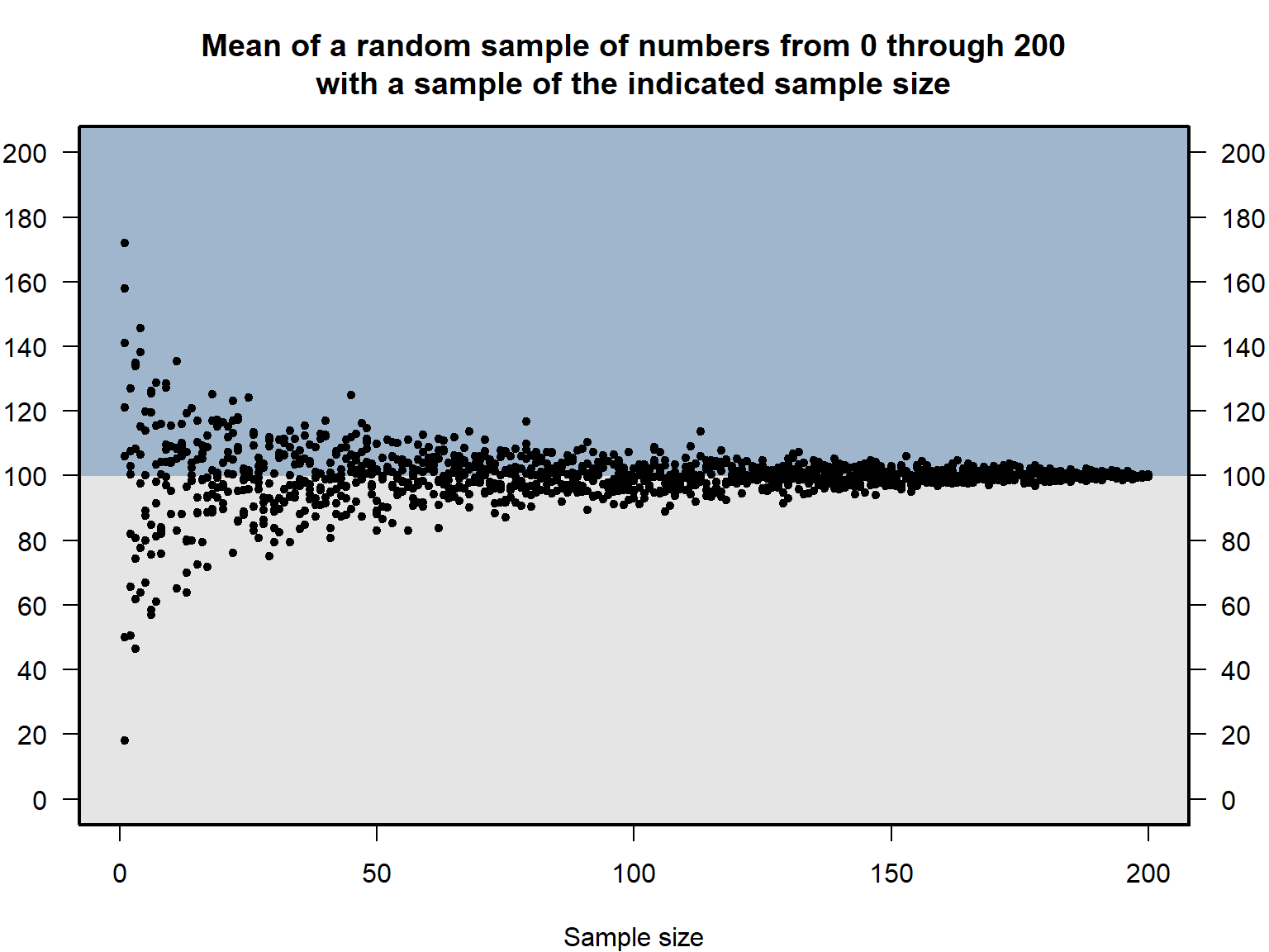
Let’s run a simulation to illustrate this. The population will be the set of whole numbers from 0 through 200, so the mean of the population is 100. The simulation will randomly draw numbers from this population and will calculate the mean of the sampled numbers. Some of the samples will be small (such as 2 or 3 sampled numbers) and some of the samples will be large (such as 100 or 150 or 200 sampled numbers). As the plot below indicates, compared to means for the smaller samples, the means for the larger samples tend to be closer to the population mean of 100.
2.3 Relatively small samples can be useful
Let’s run a few simulations to show that, even with a large population, characteristics of relatively small samples can be expected to be relatively close to the true population characteristics. Let’s use a population that has 1 million people, of whom 600,000 are female and 400,000 are male, for a population that is 60% female and 40% male. This first simulation samples 100 of the 100 million people and calculates the percentage of the sample that is female. I’ll run the simulation 5,000 times and plot the 5,000 percentages female for each of the 5,000 samples:
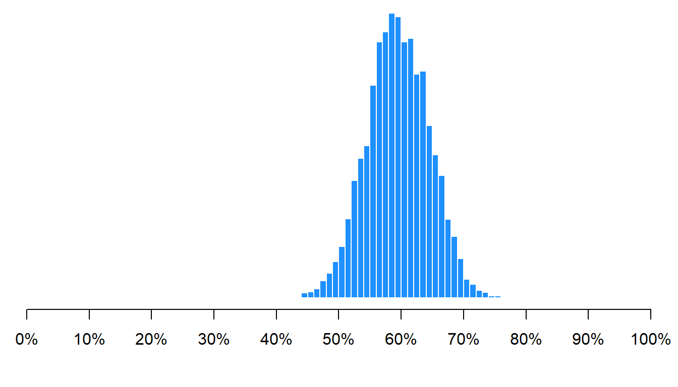
As indicated in the histogram above, the mean percentage female across all samples was 60%, which is the correct percentage female in the population. Not all samples had a percentage female that was exactly 60%, but 95% of the percentage females in the 5,000 simulated samples fell between 50% female and 70% female.
Let’s run the same simulation, but instead of sampling 100 of the 100 million people each time, let’s sample 250 of the 100 million people each time:
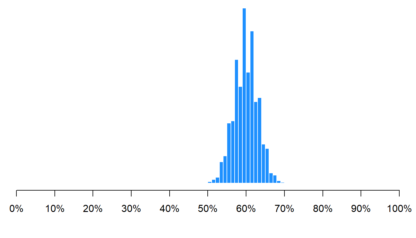
As indicated in the histogram above, the mean percentage female across all samples was 60%, which is the correct percentage female in the population. Not all samples had a percentage female of exactly 60%, but 95% of the percentage females fell between 54% female and 66% female. That’s not too bad, for sampling only 250 people from a population of 100 million.
Let’s run the same simulation, but let’s sample 1,000 of the 100 million people each time:
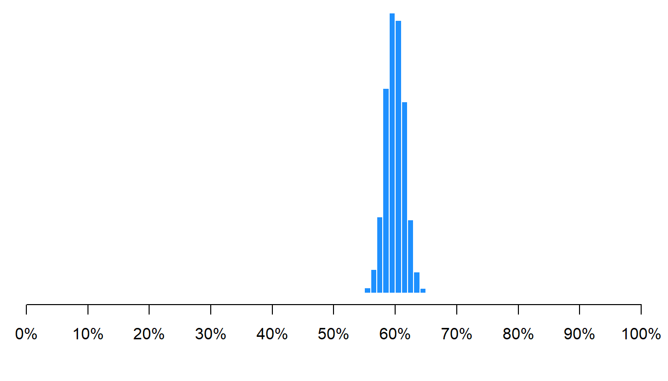
As indicated in the histogram above, the mean percentage female across all samples was 60%, which is the correct percentage female in the population. Not all samples had a percentage female of exactly 60%, but 95% of the percentage females fell between about 57% female and 63% female. That’s not too bad, for sampling only 1,000 people from a population of 100 million.
2.4 Sampling weights
The Law of Large Numbers indicates that a larger random sample will on average be expected to produce a more accurate estimate of the population, compared to the estimate that is produced by a smaller random sample. However, the Law of Large Numbers does not mean that a larger non-random sample will be expected to be more accurate than a smaller non-random sample is. The key feature for the Law of Large Numbers is that the samples are random. For instance, if Fox News had a poll on their website measuring support for Republicans, results from that poll would likely not be an accurate sample of the U.S. population, even if the sample for the poll had millions of U.S residents. Persons who visit the Fox News website are plausibly more Republican on average compared to the typical U.S. resident, so the poll would likely be biased to overestimate support for Republicans.
Remember that a population is the set of things of interest for a study, and a sample is the set of things that were studied for the study. Researchers have tools to address samples that are not representative of their population on relevant characteristics. For example, about 16% of the U.S population is Hispanic, but we might have a sample in which only 8% of the sample is Hispanic. For this, we can apply sampling weights. For these weights, we can multiply each observation by a number that represents whether the observation is overrepresented, underrepresented or correctly represented. Let’s use race/ethnicity as an example, for a hypothetical sample:
| Population % | Sample % | Sampling Weight | Sampling Weight | |
|---|---|---|---|---|
| Non-Hispanic White | 63 | 60 | 63 / 60 | 1.050 |
| Non-Hispanic Black | 13 | 13 | 13 / 13 | 1.000 |
| Hispanic | 16 | 8 | 16 / 8 | 2.000 |
| Non-Hispanic Asian | 6 | 8 | 6 / 8 | 0.750 |
| Other | 2 | 11 | 2 / 11 | 0.182 |
The sampling weight for a group is calculated by dividing the population representation by the sample representation. For this example, Hispanics are 16% of the population and 8% of the sample, so the weight for each Hispanic in the sample would be 2, if weights were only used for race/ethnicity. We multiply each Hispanic observation in the sample by 2, to get the sample Hispanic of 8% to equal the population Hispanic of 16%.
The survey weight formula in general is:
\[\text{Survey weight}=\frac{\text{% in the population}}{\text{% in the sample}}\]
Generally speaking, if a person is underrepresented in the sample, then the sampling weight will be greater than 1, because multiplying by a number greater than 1 will increase the emphasis on that observation. And if a person is overrepresented in the sample, then the sampling weight will be less than 1, because multiplying by a number less than 1 will increase the emphasis on that observation. And if a person is correctly represented in the sample, then the sampling weight will be 1, because multiplying by 1 will not change the emphasis on that observation.
Survey weights often account for multiple factors, such as gender, race, ethnicity, education, and income. The survey weight logic applies when the weights address more than one factor. For example, if Black women are 6% of our population and are 4% of our sample, then the survey weight that gets applied to each Black women in the sample would be 6/4 or 1.5.
Researchers can use weights to address differences between sample characteristics and population characteristics, if the sample characteristics and population characteristics are known or can be plausibly estimated. For example, if we know from U.S. Census data that about 13% of the U.S. population is Black, and we ask participants in our survey to indicate their race, then we can use weights to address differences in the sample percentage Black and the population percentage Black.
But we sometimes don’t have good data on particular characteristics of a population. For example, we might not have a good sense of the percentage of the U.S. population that is a conspiracy theorist, so if conspiracy theorists are less likely to take our survey, we might misestimate characteristics of the population that are correlated with being a conspiracy theorist, because – without good population estimates of the percentage of conspiracy theorists in the population – we can’t be sure of how good our weights are for any weights that we calculate for conspiracy theorists.
Sample practice items
Researchers might want to weight survey data…
- when the sample is too large
- when the population is homogeneous
- when sample characteristics do not match the population characteristics
- when the p-value for a test of the null hypothesis is not less than p=0.05
Answer
- when sample characteristics do not match the population characteristics
Suppose that, for a survey, 70% of the sample is female and 55% of our population is female. The survey weight applied to females in this case should be…
- 70/55
- 55/70
- 30/45
- 45/30
Answer
- 55/70
If the mean survey weight for a group is 0.4, then that means that the group was…
- undersampled, relative to the group’s percentage of the population
- oversampled, relative to the group’s percentage of the population
- neither undersampled nor oversampled, relative to the group’s percentage of the population
Answer
- oversampled, relative to the group’s percentage of the population
A weight of 1 does not change the group’s weight. A weight above 1 increases the group’s contribution to the population estimate, and a weight under 1 reduces the group’s contribution to the population estimate.
2.5 Confidence intervals
A 95% confidence interval can be conceptualized as a range of plausible values for an estimate. A more precise conceptualization for a 95% confidence interval for the mean of a sample is that, if we random sampled from a population over and over again and calculated a 95% confidence for the mean for each sample, 95 percent of these 95% confidence intervals would contain the true population mean.
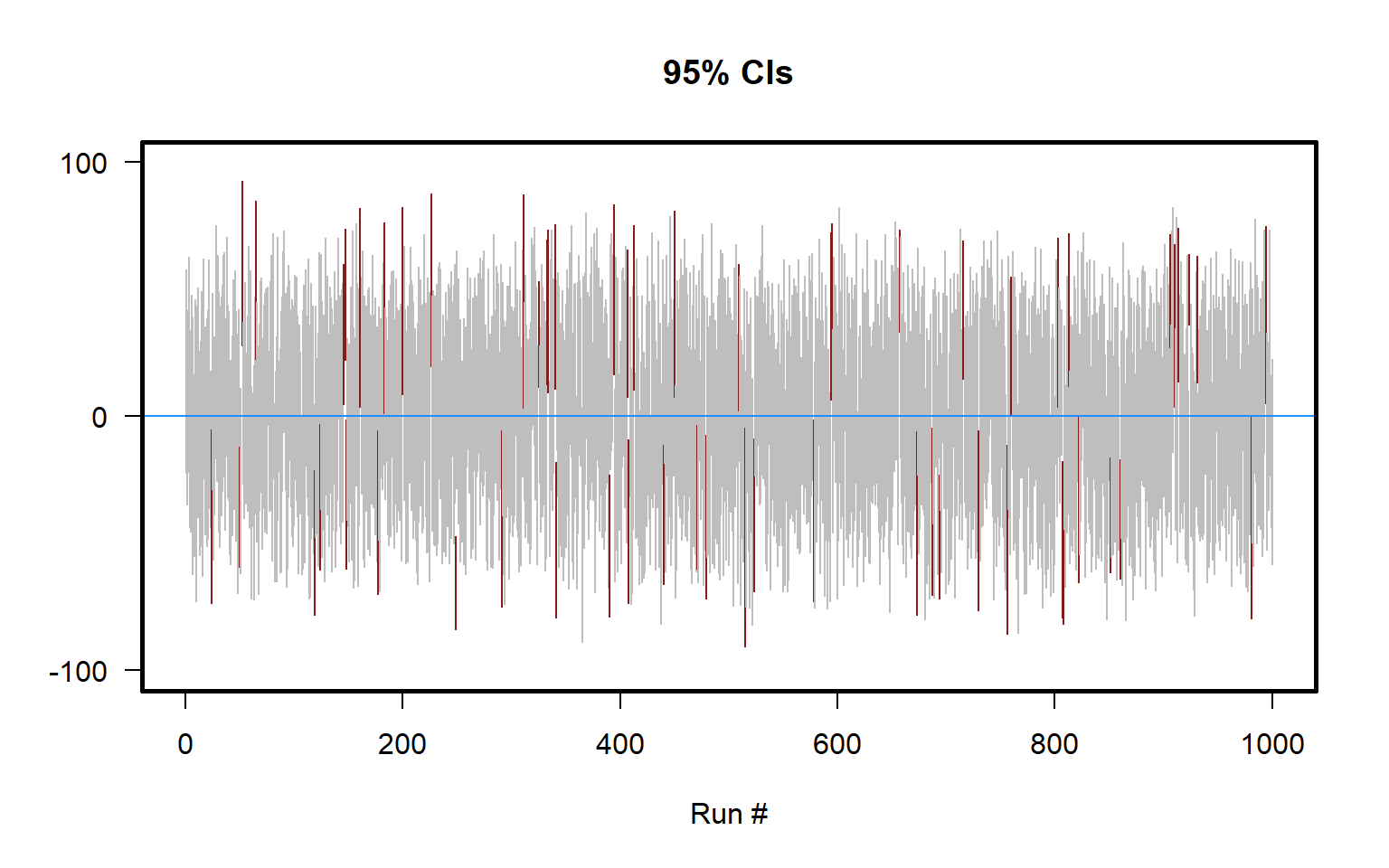
Let’s illustrate that with a simulation in the figure below, which plots 95% confidence intervals for samples of size n=10 drawn from a set of integers from -100 to +100. The 95% confidence intervals that contain the true population mean of zero are colored gray, and the 95% confidence intervals that do not contain the true population mean of zero are colored red. As illustrated in the plot, about 95 percent of the 95% confidence intervals contain the true population mean.
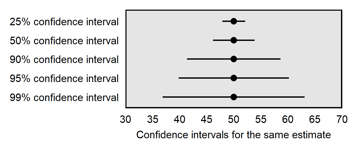
Sometimes percentages other than 95% are used to construct confidence intervals. The higher the percentage for a confidence interval, the wider the confidence interval must be to contain the true population mean. For example, a 99% confidence interval must contain the true mean 99 percent of the time, so a 99% confidence interval must be wider than a 95% confidence interval. And, the lower the percentage for a confidence interval, the thinner the confidence interval will be, all else equal.
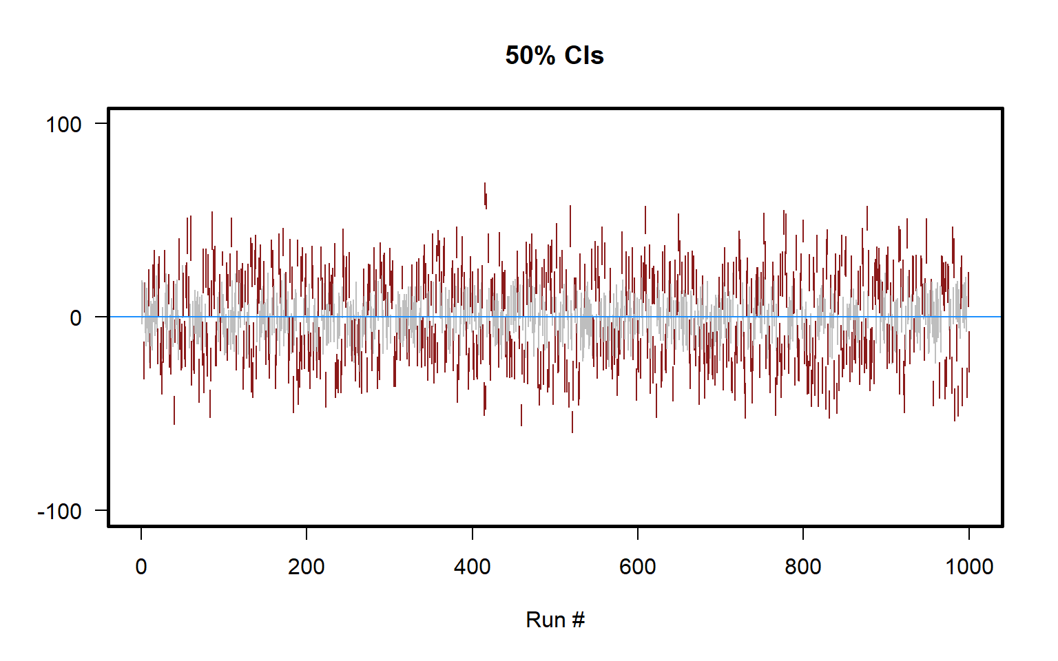
Below is a plot for 50% confidence intervals for the above situation of samples of size n=10 drawn from a set of integers from -100 to +100. The plot indicates that only about 50 percent of the 50% confidence intervals contain the true estimate (only about half of the lines are gray), and the plot also indicates that the 50% confidence intervals are not as wide as the 95% confidence intervals are for the same estimate.
Below is a plot of different confidence intervals for 50 heads in 100 flips, illustrating how having a higher confidence level requires a wider range of estimates.
So one factor that influences the width of a confidence interval is the associated percentage, such whether the confidence interval is a 95% confidence interval or a 50% confidence interval. Another factor that influences the width of a confidence interval is the data that are used to construct the confidence interval. One of these factors about the data is the sample size of the data: all else equal, larger samples produce thinner confidence intervals, because a larger amount of data from random sampling better helps us “close in” on the true characteristic of the population.
The plot below illustrates how larger samples produce thinner confidence intervals, all else equal. For the plot, the underlying data are flips of a fair coin. The top row is for 10 flips that produced 5 heads and 5 tails, the second row is for 20 flips that produced 10 heads and 10 tails, and so forth.
| SAMPLE SIZE | 95% CONFIDENCE INTERVAL |
|---|---|
| 10 flips | [19%, 81%] |
| 20 flips | [28%, 72%] |
| 100 flips | [40%, 60%] |
| 200 flips | [43%, 57%] |
| 1,000 flips | [47%, 53%] |
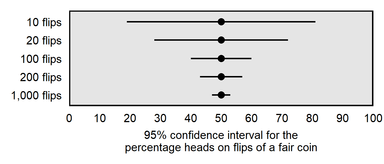
Notice that, in terms of reducing the width of the 95% confidence interval, adding 10 flips to 10 flips was more useful than adding 100 flips to 100 flips. This reflects the fact that, as sample size increases, a extra observation is not as useful as prior observations have been.
Sample practice items
For a given estimate, all else equal, which one of the following would be the widest?
- 90% confidence interval
- 95% confidence interval
- 99% confidence interval
Answer
- 99% confidence interval
Amy randomly samples 30 ISU students and asks them to rate the president on a scale from 0 for very cold to 100 for very warm. Bob randomly samples 200 ISU students and asks them to rate the president on a scale from 0 for very cold to 100 for very warm. Which of the following, if any, should be expected due to this difference in sample size?
- The mean support for the president is lower in Amy’s sample than in Bob’s sample.
- The mean support for the president is higher in Amy’s sample than in Bob’s sample.
- Neither of the above
Answer
- Neither of the above
Amy randomly samples 30 ISU students and asks them to rate the president on a scale from 0 for very cold to 100 for very warm. Bob randomly samples 200 ISU students and asks them to rate the president on a scale from 0 for very cold to 100 for very warm. Which of the following, if any, should be expected due to this difference in sample size?
- The 95% confidence interval for mean support for the president is thinner in Amy’s sample than in Bob’s sample.
- The 95% confidence interval for mean support for the president is thinner in Bob’s sample than in Amy’s sample.
- Neither of the above
Answer
Bob has more data than Amy has, all else equal, so:(B) The 95% confidence interval for mean support for the president is thinner in Bob’s sample than in Amy’s sample.
2.6 Margin of error
Surveys sometimes report an estimate plus or minus a particular number, such as 50% \(\pm\) 3%. If the confidence interval isn’t explicitly indicated for an estimate, a plausible assumption is that the calculation was based on a 95% confidence interval, so 50% \(\pm\) 3% would indicate a 95% confidence interval of [47%, 53%].
Below is a formula that can be used to estimate a margin of error for a mean measured from a large random sample, using a 95% confidence interval, in which s is the sample standard deviation and n is the sample size. Standard deviation is in the numerator, so, all else equal, a larger standard deviation produces a larger margin of error. Sample size is in the denominator, so, all else equal, a larger sample size produces a smaller margin of error.
\[ MOE = 1.96 \times \frac{s}{\sqrt{n}} \] Below is a formula that can be used to calculate a margin of error for a proportion measured from a large random sample, using a 95% confidence interval, in which p is the sample proportion and n is the sample size:
\[ MOE = 1.96 \times \sqrt{\frac{(p)(1-p)}{n}} \] For a formula that uses percentages (from 0 to 100) for p instead of proportions (from 0 to 1):
\[ MOE = 1.96 \times \sqrt{\frac{(p)(100-p)}{n}} \]
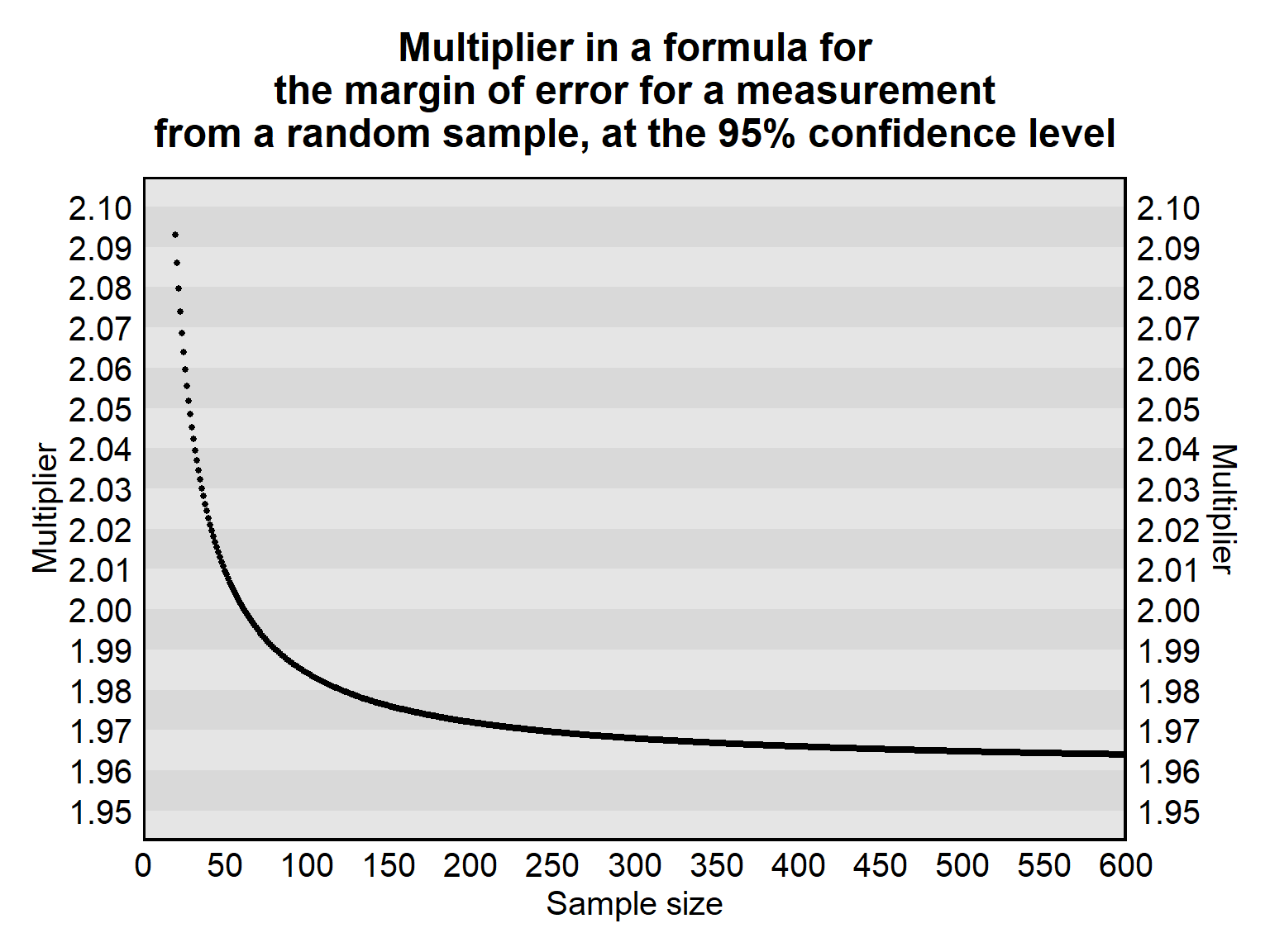
The front number 1.96 in the above formulas is the multiplier for a margin of error for a 95% confidence interval for a large sample. The multiplier that is used in a formula depends on the confidence interval percentage and the sample size. For example, the formula for the margin of error for a mean measured from a large random sample using a 99% confidence interval is:
\[ MOE = 2.58 \times \frac{s}{\sqrt{n}} \] If the margin of error is for a 95% confidence interval but the sample size is only 10, then the formula is:
\[ MOE = 2.26 \times \frac{s}{\sqrt{n}} \]
Tables are available online and elsewhere to determine the correct multiplier for a margin of error formula, but, for this course, you will be given or referred to the appropriate formula. As indicated in the plot below, for a margin of error at the 95% confidence level, the multiplier is close to 1.96 for relatively large samples.
Such formulas used to calculate a margin of error are for random samples in which the only source of error is random sampling error. But sometimes some researchers use these formulas for samples that are not random. Using one of these margin of error formulas if the sample is not random can plausibly produce underestimates of the margin of error for an estimate, because a non-random sample plausibly has more sampling error than a random sample has.
Sample practice items
Suppose that, in a random sample of 256 Illinois residents, the mean rating about the governor on a scale from 0 to 100 was 68, and the standard deviation of the ratings was 24. Use the margin of error formula below to calculate the margin of error for the mean rating of the governor, in which s is the sample standard deviation and n is the sample size.
\[ MOE = 1.960 \times \frac{s}{\sqrt{n}} \]Answer
\[ MOE = 1.960 \times \frac{24}{\sqrt{256}} = 2.94 \] So the margin of error for the mean rating is 2.94. So the estimated mean rating in the population is 68 \(\pm\) 3, if rounding to the nearest whole number.Use the margin of error formula below to calculate the margin of error for an estimated percentage of persons who approve of the governor in a population, based on a random sample of the population in which 300 of 500 residents approved of the governor, in which p is the sample percentage and n is the sample size:
\[ MOE = 1.960 \times \sqrt{\frac{(p)(100-p)}{n}} \]