7 Quasi-random designs
7.1 Natural experiments
A natural experiment is similar to a randomized experiment, but, in a natural experiment, nature assigns the treatment in a way that is random or at least is close to random. For example, some studies estimate the effect of having an extra child, by comparing women who give birth to twins to women who give birth to a singleton child. In many or most cases, having twins is random enough, so that, on average, there should not be substantial differences between women who give birth to a singleton child and women who give birth to twins.
Another natural experiment was used to assess the extent to which selling alcohol at baseball games influenced the amount of crime in the area after the game. By rule, a particular baseball team stopped selling alcohol at home games after the seventh inning. Most baseball games end after nine innings, so some fans are still drunk at the end of the game. But some games go into extra innings, so, if a game does not end until, say, the 15th inning, then the fans haven’t had alcohol in a long time and thus are no longer drunk. This might not be a perfect randomized experiment: for example, a good team like the New York Yankees is presumably more likely to go into extra innings against another equally-matched good team like the Houston Astros than against a bad team like the Detroit Tigers, and maybe fans at the Astros game are more or less likely to drink to drunkenness than fans at the Tigers game. But this might be such a small concern that this natural experiment is close enough to a randomized experiment to be useful for making causal inferences.
Let’s look at another example, from Bleakley and Ferrie 2016. The plot below is from non-experimental data, indicating that, compared to fathers in 1850 Georgia who had a low percentile of total wealth, fathers in 1850s Georgia who had a higher percentile of total wealth were much more likely to send their children to school. Data in the figure are cross-sectional, which means that we only observe father/son combinations at one point in time. Differences between points along the X-axis are not jumps in an individual father’s wealth, but are instead differences in wealth between different fathers at the same point in time.
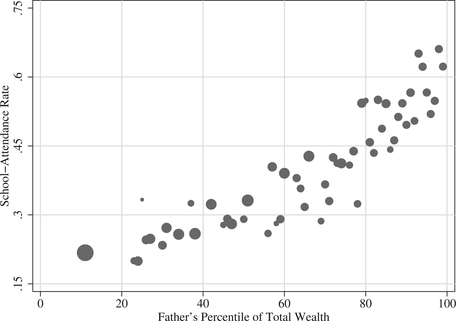
One potential explanation for this pattern is that being wealthy caused fathers to be more likely to send their children to school. But another potential explanation is that the factors that caused a father to be wealthy also caused the father to be more likely to send their children to school. The problem with correlational data is that correlational data cannot help us decide between these competing explanations.
But Bleakley and Ferrie 2016 analyzed data from an 1832 lottery in Georgia that permitted stronger causal identification. This lottery provided winners about $700, which was a substantial amount of wealth, close to median wealth at the time. Bleakely and Ferrie 2016 compared outcomes for fathers who won the lottery to outcomes for fathers who were eligible to win the lottery but did not win the lottery. The benefit of comparing lottery winners to lottery losers is that these groups should be similar to each other before the random “treatment” of winning the lottery. For example, the mean age was 51.3 among lottery losers and was 50.9 among lottery winners, the percentage that couldn’t read and write was 14.7% among lottery losers and 14.2% among lottery winners, and the number of children born within the three years prior to the lottery was 1.333 for lottery losers and was 1.332 for lottery winners.
Bleakley and Ferrie 2016 checked to see whether winning of the lottery had affected winners’ wealth in 1850, which was 18 years after the lottery. The total wealth was $3,876.50 among winners and was $3,245.50 among losers, which was a $631 difference, and the corresponding p-value of p=0.006 lets us infer that these total mean wealths differed from each other. However, as measured after the lottery, the school attendance rate among the children of lottery winners was almost identical to the school attendance rate among lottery losers: 34.2% for losers and 34.1% for winners (p=0.799). This experimental result strongly suggests that the correlation in the figure was not a causal association.
7.2 Discontinuity designs
A discontinuity design compares observations just below a threshold that received a treatment, to observations just above the threshold that did not receive the treatment. The presumption is that, compared to observations just below the threshold, observations just above the threshold are reasonably similar on all relevant characteristics other than receiving the treatment, so that the only major difference between the groups is the receipt of the treatment.
For example, suppose that we are interested in whether a college student being assigned to an honors program at that college increases that student’s income in their first year after college. Let’s illustrate this below, with hypothetical data for students at a college in which each student who has a 3.0 GPA or higher is in the honors program and no other student at the college is in the honors program. The red dots represent the students who have a GPA below 3.0 and who are thus not in the honors program, and the green dots represent the students who have a GPA of 3.0 or higher and who are thus in the honors program…
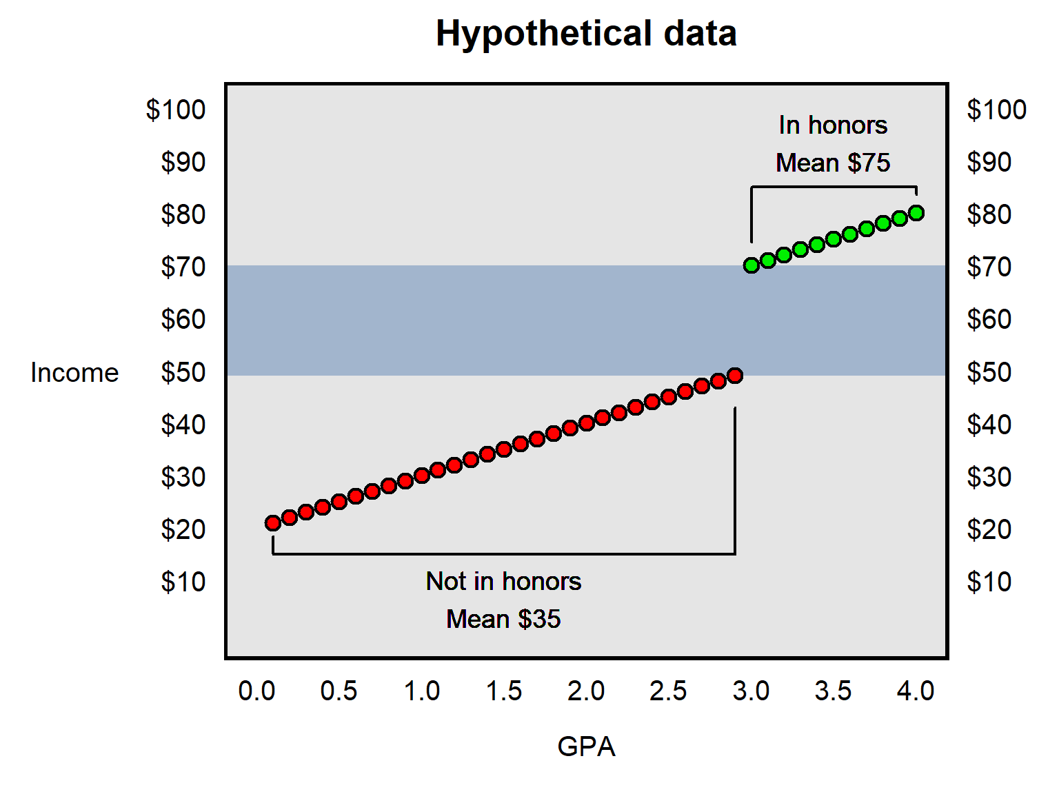
One bad way to estimate the effect of being in the honors program is to compare the mean income for the honors students ($75) to the mean income for the non-honors students ($35) and then estimate that the effect of the honors program is a $40 increase in income. This flaw in that reasoning is that a lot of that $40 gap might be attributed to factors other than the honors program; for example, in our hypothetical, the mean GPA is about 3.5 among honors students and only about 1.5 among non-honors students, so maybe the $40 gap is due to factors such as intelligence and conscientiousness that might cause student differences in GPA.
For a discontinuity design, we might instead compare the income among students who were just below the threshold to get into the honors program ($49, in our hypothetical, at a 2.9 GPA) to the income among students who were just above the threshold to get into the honors program ($70, in our hypothetical, at a 3.0 GPA), to estimate that the effect of the honors program is about a $21 increase in income. The logic of this more restricted comparison is that – other than being in a honors program – a non-honors student with a 2.9 GPA is presumably relatively similar on all relevant factors to a honors student with a 3.0 GPA, compared to how similar a typical non-honors student is to a typical honors student.
The discontinuity design has the advantage of being able to produce a plausible estimate of the treatment effect. But the limitation is that this estimate of the treatment effect is local to the threshold. In our example above, the discontinuity design will provide a plausible estimate of the effect of being in the honors program among students around the threshold for getting into the honors program. But this estimate isn’t necessarily a plausible estimate of the treatment effect on students far from the threshold.
For another example of a discontinuity design, consider the Kuipers 2022 article “Failing the Test: The Countervailing Attitudinal Effects of Civil Service Examinations”:
I surveyed the universe of recent applicants to the Indonesian civil service to study the effects of high-stakes examinations on political attitudes. Leveraging applicants’ scores on the civil service examination, I employ a regression discontinuity design to compare the attitudes of applicants who narrowly failed with those who narrowly passed. I show that the simple fact of failure on the civil service examination decreased applicants’ belief in the legitimacy of the process and levels of national identification while increasing support for in-group preferentialism.
Sample practice items
Redlining is the practice of discriminating against persons who live in “redlined” areas, such as not lending money to persons who live in redlined areas. Many redlined areas in the United States have been areas in which Blacks were disproportionately represented. Suppose that we wanted to estimate the extent to which redlining has reduced the wealth of persons who currently live in redlined areas. Explain which of these two research designs would be better:
- Compare the average wealth of contemporary U.S. residents who currently live in redlined areas, to the average wealth of contemporary U.S. residents who do not currently live in redlined areas.
- Compare the average wealth of contemporary U.S. residents who currently live at the edge of a redlined area inside the redlined area, to the average wealth of contemporary U.S. residents who currently live at the edge of a redlined area outside the redlined area.
Answer
(B), to hold more factors similar to each other.7.3 Difference-in-differences designs
Like a discontinuity design, a difference-in-differences design can be used when there is a major break in which it is plausible that the break is the only major change and thus can be considered as if it were an experimental treatment. But a difference-in-differences design includes a comparison group that, before the treatment, was similar to the group of interest and, as best we can tell, should be expected to have been similar to the treated group afterwards, if not for the difference in treatment.
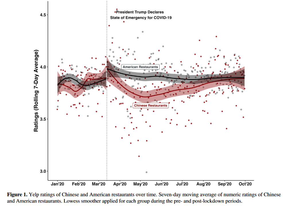
For example, the plot below from Kim and Kam 2023 indicates that, after the covid-19 emergency was declared, Yelp reviews about Chinese restaurants decreased; this seems plausibly due to anti-Chinese sentiment, because of claims that covid came from China. But the decrease is Yelp ratings for Chinese restaurants might not be particular to Chinese restaurants. After the covid declaration, most restaurants transitioned to delivery, so maybe all restaurants experienced a drop in Yelp ratings, if Yelp raters merely didn’t like eating delivery as much as eating in person. Kim and Kam 2023 addressed that potential alternate explanation by comparing the difference in Yelp ratings about Chinese restaurants before and after the covid-19 emergency was declared, to the difference in Yelp ratings about American restaurants before and after the covid-19 emergency was declared. The decrease in Yelp ratings for Chinese restaurants did not occur for American restaurants, which can give us more confidence that that decrease in Yelp ratings for Chinese restaurants was due to anti-Chinese sentiment.
Sample practice items
Suppose that, on 1 January 2018, Freedonia City put into effect a law that banned prostitution. We want to estimate how this ban affected drug crime. Before the prostitution ban, drug crime in Freedonia City had been increasing at 3% per year, but, after the prostitution ban, drug crime in Freedonia City increased at only 1% per year. Like Freedonia City, Otisburg and Luthorville are cities in Freedonia, Prostitution was legal in Otisburg and in Luthorville before and after 1 January 2018. For estimating how the Freedonia City ban on prostitution affected drug crime in Freedonia City, which of these cities would provide the better comparison for a difference-in-difference design, based on the information below?:
- Otisburg, in which drug crime was increasing at 3% per year before 1 January 2018
- Luthorville, in which drug crime was increasing at 3% per year after 1 January 2018
Answer
- Otisburg, in which (like in Freedonia City) drug crime was increasing at 3% per year before January 1, 2018
Suppose that a researcher is interested in the extent to which college causes persons to become more liberal politically. In 2019, the researcher surveys a representative sample of age-18 persons who attend college and a representative sample of age-18 persons who do not attend college; four years later, in 2023, the researcher surveys each person again. Suppose that the researcher’s data is as in the table below, in which political ideology is measured from 0 for extremely liberal to 10 for extremely conservative.
| Group | Mean ideology at age 18 | Mean ideology at age 24 |
|---|---|---|
| Persons in college | 4.5 | 3.5 |
| Persons not in college | 5.0 | 4.2 |
If the researcher analyzed only the data for persons in college, the researcher’s (incorrect) estimate of the effect of college on the political ideology of persons in the researcher’s sample would be that college…
- made persons in the sample about 0.2 units more liberal on average
- made persons in the sample about 0.8 units more liberal on average
- made persons in the sample about 1.0 unit more liberal on average
- made persons in the sample about 3.5 units more liberal on average
Answer
- made persons in the sample about 1.0 unit more liberal on average
Suppose that a researcher is interested in the extent to which college causes persons to become more liberal politically. In 2019, the researcher surveys a representative sample of age-18 persons who attend college and a representative sample of age-18 persons who do not attend college; four years later, in 2023, the researcher surveys each person again. Suppose that the researcher’s data is as in the table below, in which political ideology is measured from 0 for extremely liberal to 10 for extremely conservative.
| Group | Mean ideology at age 18 | Mean ideology at age 24 |
|---|---|---|
| Persons in college | 4.5 | 3.5 |
| Persons not in college | 5.0 | 4.2 |
If the researcher used a difference-in-differences design that compared persons in college to persons not in college, the researcher’s (more correct) estimate of the effect of college on the political ideology of persons in the researcher’s sample would be that college…
- made persons in the sample about 0.2 units more liberal on average
- made persons in the sample about 0.8 units more liberal on average
- made persons in the sample about 1.0 unit more liberal on average
- made persons in the sample about 3.5 units more liberal on average
Answer
- made persons in the sample about 0.2 units more liberal on average