17 Readings
Note: No need for students to draft responses to the items below, but the items are things that we might discuss in class when discussing the indicated reading.
Things to consider when reading Burge et al 2020
Things to consider when reading Burge et al. 2020 “A Certain Type of Descriptive Representative? Understanding How the Skin Tone and Gender of Candidates Influences Black Politics”:
[abstract] The journal Social Science Quarterly requires that a manuscript abstract discuss four things about the research: the Objective, the Methods, the Results, and the Conclusions. Does the abstract for Burge et al. 2020 include all four of these things? Does the abstract for Burge et al. 2020 include anything valuable other than these four things?
[Figure 1, 2, and 3] Do each of Figures 1, 2, and 3 clearly communicate the main finding(s) that you think the authors intended to be communicated in the figures? Can you think of any ways to improve Figures 1, 2, or 3?
[Figure 1, 2, and 3] Each figure and its note should provide enough information so that a reader does not need to refer to the main text to understand the figure. Do Figures 1, 2, and/or 3 and/or the notes for the figures need to indicate any additional information for readers to understand the figure?
[page 1598] Did Burge et al. 2020 report sufficient information in the Method section so that you can understand their research method? Can you think of any information that Burge et al. 2020 might have added to help readers better understand the method?
[page 1598] Instead of reporting exact p-values to, say, three decimal places, Burge et al. 2020 reported p-values as inequalities such as p<.5 and p<.1. Which do you think is better, and why: reporting exact p-values, or reporting p-value inequalities?
[page 1598] Burge et al. 2020 footnote 2 refers readers to the appendix for results in which experimental conditions that manipulated Black candidate skin color are compared to a control condition that did not contain a photo of the candidate or any indication of candidate skin tone. Did the research reported in Burge et al. 2020 need a control condition? If not, how can researchers correctly decide whether to include or to not include a control group?
[page 1598] Burge et al. 2020 indicated that the experimental results were analyzed with an ordinary least squares linear regression using statistical control for gender, education, income, age, self-reported skin tone, and partisanship. Strictly speaking, because of random assignment, statistical control is not needed to analyze data from a randomized experiment. But can you think of any advantage to using statistical control for analyzing data from a randomized experiment?
[page 1598] Burge et al. 2020 indicated that “Respondents were 3 percentage points more likely to vote for dark-skinned candidates”. Below is information about how the “likelihood to vote” outcome variable was measured and coded in the Stata commands, and, if you remember, a linear regression was used to analyze this outcome variable. Can you see a potential problem describing these results in terms of percentage points?
How likely are you to vote for this candidate?
o   Not at all likely
o   Slightly likely
o   Moderately likely
o   Very Likely
o   Extremely likely

. tab vote_re

    vote_re |      Freq.     Percent        Cum.
------------+-----------------------------------
          0 |         99        7.86        7.86
        .25 |        182       14.44       22.30
         .5 |        393       31.19       53.49
        .75 |        375       29.76       83.25
          1 |        211       16.75      100.00
------------+-----------------------------------
      Total |      1,260      100.00
[Figure 4] Does Figure 4 clearly communicate the main finding(s) that you think the authors intended to be communicated in the figures? Can you think of any ways to improve Figure 4? Can you think of any information that would be helpful to add to Figure 4, presuming that figures and tables should be self-contained?
[Figure 4] Burge et al. 2020 presented all of its results without using a table. Would the presentation of results have been better replacing at least one of the figures with a table?
[general] Burge et al. 2020 mentions prior research on Blacks’ evaluation of lighter-skinned Black candidates relative to darker-skinned Black candidates, such as Lerman et al. 2015 and Brown and Lemi 2019. How did Burge et al. 2020 differentiate Burge et al. 2020 from these prior publications?
[general] What did Burge et al. 2020 suggest is the key contribution of Burge et al. 2020?
[general] Burge et al. 2020 wrote that its argument is (p. 1598)…
“…that the perceived discrimination and other lived experiences of dark-skinned Black candidates leads them to be preferable to Black voters who want descriptive representatives who understand and can address the needs of the racial group”.
How, if at all, did Burge et al. 2020 test the argument that perceived discrimination and other lived experiences cause Black participants to prefer dark-skinned Black candidates to light-skinned Black candidates?
[general] Suppose that the Burge et al. 2020 results had indicated that Black participants preferred light-skinned Black candidates to dark-skinned Black candidates. Can you think of a theory that would explain that pattern?
[Don’t worry about this for now, but I’m putting this here as a reminder for me to discuss this in class] Burge et al. 2020 (p. 1598) indicates that the p-value is p<.05 for Figure 1 and Figure 3. However, the 95% confidence intervals overlap in Figure 1 and Figure 3. If the 95% confidence intervals overlap, is it possible that the p-value is p<.05 for a test of the null hypothesis that the mean for the light-skinned candidate differs from the mean for the dark-skinned candidate? See the output below for Figure 1, based on Burge et al. 2020 code:
. ttest vote_re if tonegroup==2|tonegroup==3, by(tonegroup)

Two-sample t test with equal variances
------------------------------------------------------------------------------
   Group |     Obs        Mean    Std. Err.   Std. Dev.   [95% Conf. Interval]
---------+--------------------------------------------------------------------
Light Im |     428    .5817757    .0140376    .2904122    .5541843    .6093671
Dark Ima |     411    .6216545      .01387    .2811877    .5943894    .6489196
---------+--------------------------------------------------------------------
combined |     839    .6013111    .0098895    .2864555    .5818999    .6207223
---------+--------------------------------------------------------------------
    diff |           -.0398788    .0197469               -.0786381   -.0011195
------------------------------------------------------------------------------
    diff = mean(Light Im) - mean(Dark Ima)                        t =  -2.0195
Ho: diff = 0                                     degrees of freedom =      837

    Ha: diff < 0                 Ha: diff != 0                 Ha: diff > 0
 Pr(T < t) = 0.0219         Pr(|T| > |t|) = 0.0438          Pr(T > t) = 0.9781
clear all
set obs 100000
gen group1 = _n
gen group2 = _n + 253
ttest group1 = group2, unp une
ttest group1 = group2, unp une level(83.4)
ttest group1 = group2, unp une level(83)
ttest group1 = group2, unp une level(84)
Let’s discuss flaws in the Burge et al 2020 figure below, which include:
- Information for the outcome variable is placed in the legend, but this unnecessary causes readers to need to decipher the dot, triangle, and X symbols.
- The y-axis text is vertical, which is more difficult to read than horizontal text.
- The panels are a lot taller than needed, so the top estimate is farther from the x-axis labels than needed.
- The estimates of interest unnecessarily consume too little of the plot space.
- Can you tell what central point the plot is intended to communicate to the readers?
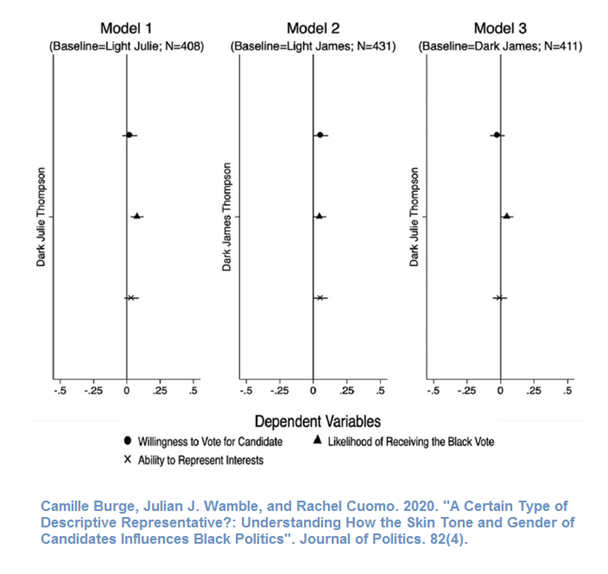
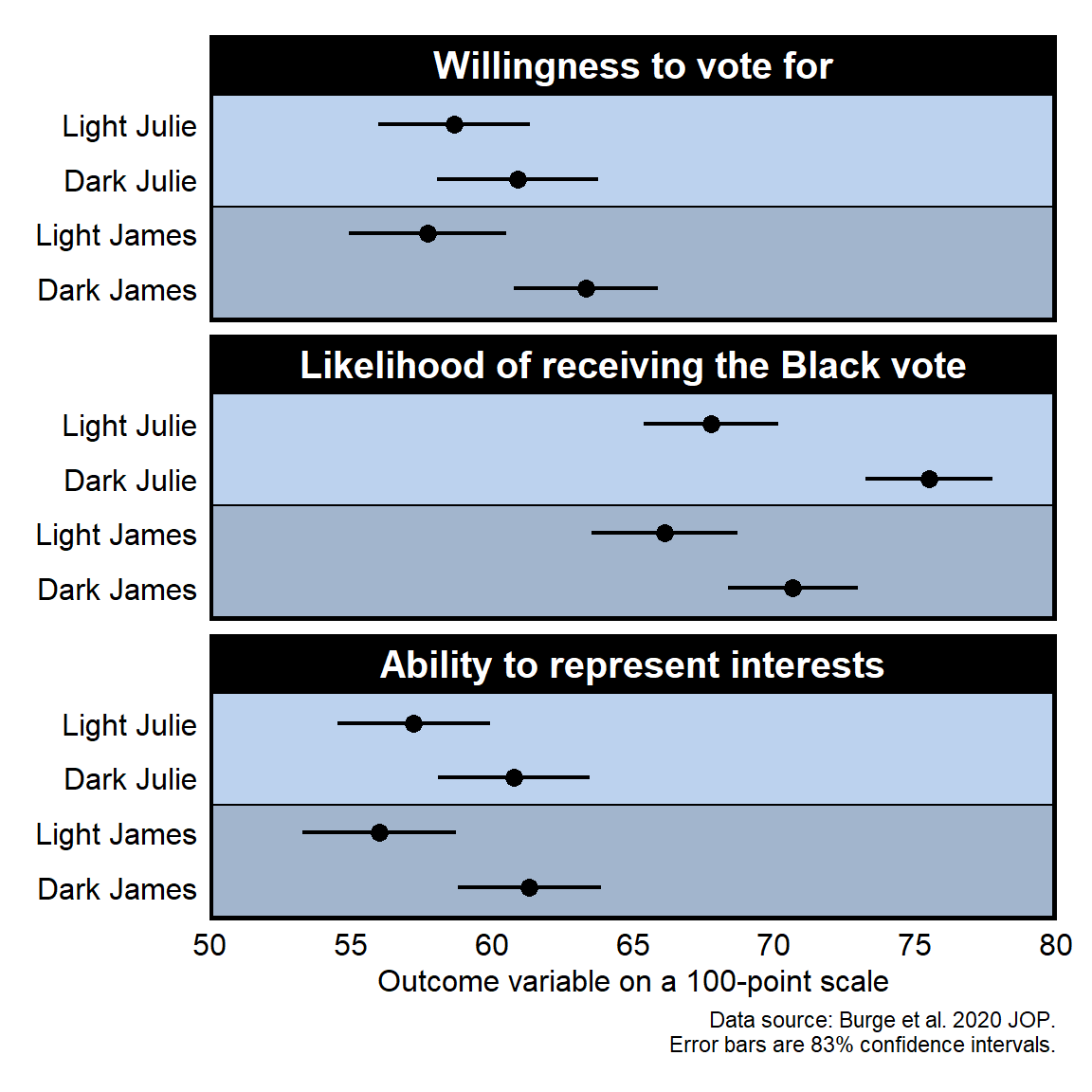
Below is a suggested revision:
Things to consider when reading Primm et al 2010
Things to consider when reading Primm et al. 2010. “The Role of Race in Football Card Prices”. Social Science Quarterly 91(1): 129-142:
[title] Do you think the title would be better if the title indicated the main finding? Something such as “Lack of Evidence that Player Race Influences Football Card Prices”?
[abstract] Based on the objective in the abstract, what is the contribution of the study to the literature?
[abstract] Data in Primm et al. 2010 are only football cards, but how does the “Conclusions” section of the abstract indicate a conclusion beyond football card prices?
[page 130] Primm et al. 2010 discussed “intangible” factors that affect a card’s value, such as the player’s off-the-field behavior. How, if at all, does the Primm et al. 2020 account for how a player’s off-the-field behavior affects the value of the player’s card?
[page 132] Primm et al. 2010 used football cards only between 1946 and 1988. How, if at all, does Primm et al. 2010 justify starting the analysis in 1946 and ending the analysis in 1988?
[page 132] Primm et al. 2010 used football cards only for Pro Bowl players (i.e., players who were considered at or near the top of their position in at least one year), but Primm et al. 2010 does not justify this limitation to the data analysis. Do you expect that the omission of cards for players who did not make a Pro Bowl will cause Primm et al. 2010 to underestimate any racial bias, overestimate any racial bias, not affect the estimate of racial bias, or have an unpredictable effect on the estimate of racial bias?
[page 133] Primm et al. 2010 did not predict the dollar value of the cards but instead predicted the log of the dollar value of the cards. How, if at all, does Primm et al. 2010 justify transforming the outcome variable to a log scale?
miscellany For transforming the outcome variable to a log scale, why was it important that no card value was exactly zero dollars?
[page 133] Primm et al. 2010 indicated that “The race of player was determined by a visual inspection of each player’s photograph as it appears on the HOF [Hall of Fame] website and in Topps Football Cards: The Complete Picture Collection” (p. 133). Is this a good way to code the race of the players? If not, what would be a better way to code the race of the players?
[Table 1] Primm et al. 2010 selected offensive lineman as the player position to omit, so that the estimates for the other positions are relative to offensive lineman; for example, the 0.065 coefficient for defensive back is the estimated difference in the outcome between a defensive back and an offensive lineman net of controls, and the lack of a statistical significance star indicates that there is insufficient evidence to conclude that a difference of this 0.065 size would be unlikely to be due to chance if there were no true difference in the mean outcome between offensive lineman and defensive backs. Why might Primm et al. 2010 have selected offensive lineman as the player position to omit?
[Table 1] Primm et al. 2010 used “Race” as the name of the variable for the race of the player. What might have been a better name for that variable?
[Table 1] Generally, it is good to report multiple models to permit the reader to get a sense of how much the key estimate changes with different reasonable model specifications. Primm et al. 2010 reported multiple models, but can you identify a major shortcoming of their selection of alternate model specifications?
[Table 1] Does Model 4 of Table 1 contain sufficient evidence to conclude at p<0.05 that the log of the card value for linebackers is higher than the log of the card value for punters/kickers, net of controls?
[misc] The Race predictor in Model 4 does not have a p-value under p=0.05 and thus is not statistically significant, which means that the analysis does not permit us to conclude that the mean logged card value for Black players differed net of controls from the mean logged card value for White players. This is a null result, but null results can be classified as informative or uninformative, in which an informative null result permits us to conclude that, even if there is an effect, the effect is small. For example, the p-value is not under p=0.05 if a coin lands on heads 3 times in 4 flips (an uninformative null) and is not under p=0.05 if a coin lands on heads 4,999 times in 10,000 flips (an informative null). Does Primm et al. 2010 permit us to conclude whether the null is informative? If not, what information could Primm et al. 2010 have provided to permit us to assess whether the null is informative?
[misc] The analysis in Primm et al. 2010 does not permit us to conclude that racial bias influenced the value of football cards, but it’s possible that racial bias influenced some of the control variables. For example, maybe racial bias unfairly kept some players from being named to the Pro Bowl or the Hall of Fame. Should this potential bias in the controls affect our interpretation of the Primm et al. 2010 null result, and, if so, why?
[misc] Primm et al. 2010 concluded by suggesting future research topics such as the effect of skin tone. Did anything stop Primm et al. from including skin tone as a predictor?
[misc] Let’s plan to discuss in class what is occurring in the simulation below:
. clear all
. set cformat %9.2f
. set seed 1234
. set obs 10000

. gen black      = round(runiform(0,1))
. gen marketsize = 2.0*black            + runiform(-2,2) + 2
. gen cardvalue  = 0.5*marketsize       + -0.1*black     + runiform(-2,2) + 2

. sum

    Variable |        Obs        Mean    Std. Dev.       Min        Max
-------------+---------------------------------------------------------
       black |     10,000       .5027    .5000177          0          1
  marketsize |     10,000    2.991714    1.515072   .0014036   5.999578
   cardvalue |     10,000    3.449911    1.360711   .0528942   6.849223

. reg cardvalue black

      Source |       SS           df       MS      Number of obs   =    10,000
-------------+----------------------------------   F(1, 9998)      =   1140.67
       Model |  1895.90317         1  1895.90317   Prob > F        =    0.0000
    Residual |  16617.5853     9,998  1.66209095   R-squared       =    0.1024
-------------+----------------------------------   Adj R-squared   =    0.1023
       Total |  18513.4885     9,999    1.851534   Root MSE        =    1.2892

------------------------------------------------------------------------------
   cardvalue |      Coef.   Std. Err.      t    P>|t|     [95% Conf. Interval]
-------------+----------------------------------------------------------------
       black |       0.87       0.03    33.77   0.000         0.82        0.92
       _cons |       3.01       0.02   164.76   0.000         2.98        3.05
------------------------------------------------------------------------------

. reg cardvalue black marketsize

      Source |       SS           df       MS      Number of obs   =    10,000
-------------+----------------------------------   F(2, 9997)      =   1949.61
       Model |  5194.80062         2  2597.40031   Prob > F        =    0.0000
    Residual |  13318.6878     9,997  1.33226846   R-squared       =    0.2806
-------------+----------------------------------   Adj R-squared   =    0.2805
       Total |  18513.4885     9,999    1.851534   Root MSE        =    1.1542

------------------------------------------------------------------------------
   cardvalue |      Coef.   Std. Err.      t    P>|t|     [95% Conf. Interval]
-------------+----------------------------------------------------------------
       black |      -0.11       0.03    -3.76   0.000        -0.17       -0.05
  marketsize |       0.50       0.01    49.76   0.000         0.48        0.52
       _cons |       2.01       0.03    77.73   0.000         1.96        2.06
------------------------------------------------------------------------------
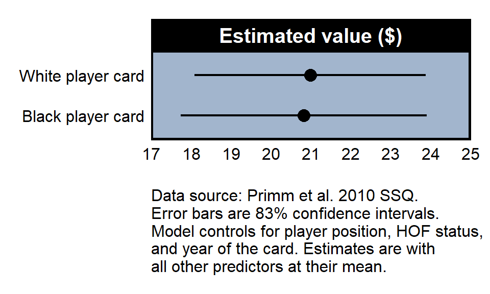
Suggested visualization for the key outcome:
Comparison of Burge et al 2020 and Primm et al 2010
For a randomized experiment, the treatment is independent of each characteristic of the participants, except for any association due to random error. There is no reason to expect that men are more likely than women to get the treatment, or that Asians are more likely than Hispanics to get the treatment, or that Republicans are more likely than Democrats to get the treatment than Democrats. Therefore, the only potential explanations for a treatment effect are [1] the treatment caused the effect and [2] random assignment error.
But for an observational study that did not involve random assignment to the treatment, the treatment might be dependent of one or more characteristic of the participants.
For example, in the Primm et al 2010 study about racial bias in football card values, the treatment is race, which we can think of as being Black relative to White or being White relative to Black. But this treatment was not randomly assigned to the football cards. For example, the “White” treatment was more likely to be assigned to older cards. Therefore, if older football cards are valued more than more recent football cards, we must address the extent to which this is due to the age of the older cards compared to being due to the older cards having a higher percentage of White players.
Statistical control is one way to address this non-random assigned of the treatment.
The logic of statistical control is to hold other relevant factors constant. So instead of comparing the mean price for Black player cards to the mean price for White player cards, we can control for the alternate explanation of the age of the card like this:
Compare the mean price for Black player cards to the mean price for White player cards, for cards from 1960…and then for cards from 1961…and then for cards from 1962…and then for cards from 1963…[etc]…and then for cards from 2000. Then we average across all of these comparisons to assess the pattern controlling for the age of the card…
Below is a graph for the difference in value between the White players’ cards and the Black players’ cards for each year.
Error in if (axes) {: the condition has length > 1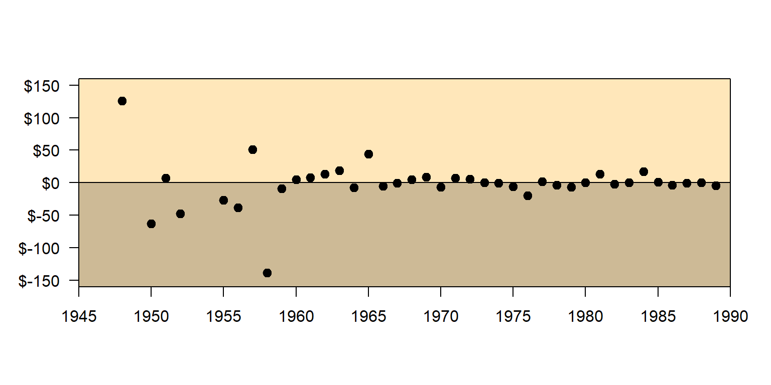
The first dot on the left indicates that, in that year, White players’ cards are on average worth about $120 more than Black players’ cards. The next dot to the right indicates that, in the next year, White players’ cards are on average worth about $65 less than Black players’ cards. Over time, there is not much relationship between the race of the player and card value, when controlling for year of the card.
Things to consider when reading Macdonald 2021
Things to consider when reading Macdonald 2021. “The Authoritarian Predisposition and American Public Support for Social Security” in Political Research Quarterly:
[page 4] The key outcome variable was measured with an item that asked participants to indicate their opinion about whether federal spending on Social Security should be increased, decreased, or kept about the same. However, the main results are reported for the outcome coded so that 1 is increased and 0 is [decreased or kept about the same]. Footnote 7 indicates that results are substantively similar if the three-part coding is used. Which of the codings (the dichotomous 0-or-1 coding or the three-part coding) is preferable, and why?
[page 4] Macdonald 2021 indicated that “I also account for economic self-interest by controlling for whether a respondent is likely to be in the ‘target population’ to receive Social Security”. Macdonald 2021 did this using three controls: a control for coded 1 for age 62+ and 0 otherwise, a control coded 1 for retired and 0 otherwise, and a control coded 1 for permanently disabled and 0 otherwise. Consider whether using these three controls would have been better or worse than using a single control coded 1 if the respondent was age 62 or older or retired or permanently disabled, and 0 otherwise.
[page 4] Macdonald 2021, discussing the coding of the ideology predictor, indicated that “To avoid dropping cases, I code respondents who indicated that they ‘hadn’t thought much’ about their ideological identification at the midpoint value of ‘4’ (Kinder and Kalmoe 2017)”. But this coding means that the respondents who selected “hadn’t thought much” for the ideology item were coded the same as the respondents who selected “moderate” for the ideology item. How could responses to the ideology item be coded to avoid coding both of these responses into the same category?
[page 5] Table 1 included year fixed effects. What are these year fixed effects? What is the value in including year fixed effects? And why would Table 1 not indicate the results for the year fixed effects?
[page 5] How did Macdonald 2021 support the claim that “authoritarianism has…a substantively…significant relationship with attitudes toward Social Security”?
[page 6] Figure 1 reports estimates for five levels of authoritarianism, with an increase from one level to the next level that appears to be the same increase for each level increase. Do the results reported in Macdonald 2021 let us infer whether this is because authoritarianism has a constant association with the outcome net of controls?
[page 6] In Figure 1, as often occurs, estimates for the middle levels of the predictor have a smaller confidence interval than estimates at the end levels of a predictor. This might be due to a larger number of observations at the middle level of a predictor. But what else might cause this pattern?
[page 6] Macdonald 2021 indicated that “I demonstrate the robustness of my main findings”. What does this “robustness” mean?
[page 7] How did Macdonald 2021 address the issue of reverse causality?
[page 8] Macdonald 2021 mentions measurement invariance. What is that?
[page 9] Macdonald 2021 indicated that:
In this article, I have shown, through analyses of cross-sectional and panel data spanning three decades, that authoritarianism is a substantively significant determinant of attitudes toward government spending on Social Security. I attribute this to the political framing of Social Security, which emphasizes themes such as ‘rule-following,’ ‘deservingness,’ and ‘certainty,’ arguing that this resonates with authoritarian-minded individuals”.
What, if any, evidence that did Macdonald 2021 provide that the framing of Social Security is the reason for the detected association?
- [misc] Below is a section of Stata output from a linear regression based on the model in Macdonald 2021 Table 1, but with separate predictors for each level of the authoritarianism measure (coded 0, 1, 2, 3, and 4) and with the middle category “2” omitted as the comparison category. The coefficient for “0” indicates that respondents at the lowest authoritarianism were 6.0 percentage points less likely to prefer increased federal spending on Social Security, net of controls, compared to respondents in omitted category “2”. The coefficient for “4” indicates that respondents at the highest authoritarianism were 6.6 percentage points more likely to prefer increased federal spending on Social Security, net of controls, compared to respondents in omitted category “2”.
Linear regression                               Number of obs     =     13,604
------------------------------------------------------------------------------
             |               Robust
     more_ss |      Coef.   Std. Err.      t    P>|t|     [95% Conf. Interval]
-------------+----------------------------------------------------------------
       auth5 |
          0  |  -.0600666   .0175158    -3.43   0.001       -.0944   -.0257333
          1  |  -.0402856    .016146    -2.50   0.013     -.071934   -.0086373
          3  |   .0274555   .0144704     1.90   0.058    -.0009085    .0558195
          4  |   .0660078   .0160418     4.11   0.000     .0345636     .097452
..............................................................................
Of the following, which is the better interpretation of these results?
- Authoritarianism caused a 12.6 percentage point increase in the probability of preferring increased federal spending on Social Security, net of controls.
- Authoritarianism caused a 6.6 percentage point increase in the probability of preferring increased federal spending on Social Security, net of controls.
Things to consider when reading Wysocki et al 2022
Some background terms are below, expressed at a simple level intended to help interpret Wysocki et al 2022.
attenuate: lessen
confounder: variable that affects a predictor and an outcome, biasing the estimate of the predictor’s effect on the outcome
endogenous: from inside the model, in the sense of not being influenced by at least one variable in the model
exogenous: from outside the model, in the sense of not being influenced by a variable in the model
instrumental variable: variable used to address an endogenous variable
nonparametric: does not require assumptions
parameter: number describing a population
parametric: require assumptions, such as a normal distribution
partial regression coefficient: regression coefficient controlling for at least one other factor
population: the set of things of interest (compare to a sample, which is limited to the set of things that are observed)
power: the ability of an analysis to detect an effect
residual: the difference between an observed outcome and the predicted outcome
simple regression coefficient: regression coefficient in the absence of other predictors
standard error of the estimated regression coefficient:
standardized: in a standard form, typically with a mean of zero and standard deviation of 1
Things to consider when reading Wysocki et al 2022 “Statistical Control Requires Causal Justification” in Advances in Methods and Practices in Psychological Science:
What do the authors mean by the title “Statistical control requires causal justification”?
What is a confounder? When, if at all, should an analysis control for a confounder?
What is a mediator? When, if at all, should an analysis control for a mediator?
What is a collider? When, if at all, should an analysis control for a collider?
What is a proxy? When, if at all, should an analysis control for a proxy?
For the right panel of Figure 1, propose variables that can plausibly be X, Y, and C. Then explain why controlling for C can help identify the causal effect of X on Y.
What is incremental validity testing?