5 Stata basics
5.1 Stata filetypes
Stat has a few types of files that we will work with:
a dta file is a Stata dataset, which can include numbers and labels for the same observation. So, for example, an observation could be coded both as the number 1 and with the label “support”, and another observation could be coded both as the number 0 and with the label “does not support”. The numbers can be used to calculate the percentage of participants who support the outcome, and the labels are useful for know what the numbers refer to.
a do file that can be used to save a set of commands and documentation indicating, for instance, what the commands are intended to do.
a log file that records the commands that are run and the output that occurs from the commands. For a log file, the smcl file type (Stata Markup and Control Language) is in Stata format, but – unless saved as a PDF or something equivalent – an smcl file cannot be read without access to Stata. The log type of log file is a text file that can be opened with a text editor that all or almost all computers should have.
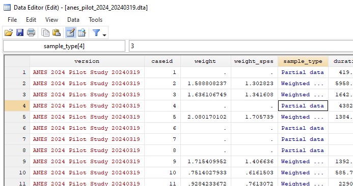
5.2 Stata data editor for cross-sectional data
Many social science datasets have only one observation for each person, country, or other thing in the dataset, with this observation taken at or around the same time. In this case, the dataset is typically st up with one observation per row. Below is an example, from the dataset for the ANES 2024 Pilot Study, in which each row is a different participant. In the Stata data editor, the red cells indicate text only cells, the black cells indicate numeric only cells, and the blue cells indicate numeric cells that have a number and an associated text label. For example, the “Partial data” label has the number 3 associated with it.
Datasets get more complicated when there are multiple observations per each person, country, or other thing. But let’s worry about that later.
5.3 Useful Stata commands
| Command | Use |
|---|---|
| edit | Open the data editor |
| lookfor | Look for text in variable names or labels |
| codebook | Get information about a variable |
| tab | Tabulate results for a variable w/options such as mi and nol |
| tabstat | Tabulate summary statistics |
| sum | Get summary statistics |
| recode | Recode a variable |
| replace | Replace levels of a variable |
| gen | Generate a new variable |
| egen | Generate a new variable using a specialized function |
| clonevar | Clone an existing variable |
| label | Label a variable (see label define, label values) |
| set cformat | Change the number of decimal places reported in regressions |
| reg | OLS linear regression |
| margins | Predicted outcomes from a regression |
| marginsplot | Plot of predicted outcomes from the margins command |
| svyset | Set up survey weights |
| svy: | Prefix for survey commands |
| logit | Regression technique for dichotomous outcomes |
Stata tips by Todd Jones
5.4 Sample Stata commands to read in data
One way to read data into Stata is to select File > Open… in the top menu and to then select the Stata file that you want to read into Stata. Stata files end with a .dta extension. You can also read in CSV and other files, using File > Import in the top menu. Or you can type “edit” into the Stata command line and then paste the data from a spreadsheet into the Stata data editor.
Let’s read in the Stata dataset for the ANES 2020 Time Series Study:
5.5 Sample Stata commands to find data
Let’s find the measure of how respondents rated police, by using lookfor to search for “police” in the variable names and variable labels but not in the variable values:
lookfor police
running D:\OneDrive - IL State University\2-teaching\R for teaching\POL497\prof

> ile.do ...

              storage   display    value
variable name   type    format     label      variable label
-------------------------------------------------------------------------------
V202171         double  %12.0g     V202171    POST: Feeling thermometer: police
V202351         double  %12.0g     V202351    POST: How often do police
                                                officers use more force than
                                                necessary
V202456         double  %12.0g     V202456    POST: During past 12 months, R or
                                                any family members stopped by
                                                police
V202491         double  %12.0g     V202491    POST: Do police treat blacks or
                                                whites better
V202492         double  %12.0g     V202492    POST: How much better do police
                                                treat blacks or whites
V202493x        double  %12.0g     V202493x   POST: SUMMARY: Police treat
                                                blacks or whites better
5.6 Sample Stata commands to describe data
Let’s get information about the V202171 measure of how respondents rated police on a 0-to-100 feeling thermometer. First, let’s use the describe command:
desc     V202171
running D:\OneDrive - IL State University\2-teaching\R for teaching\POL497\prof

> ile.do ...

              storage   display    value
variable name   type    format     label      variable label
-------------------------------------------------------------------------------
V202171         double  %12.0g     V202171    POST: Feeling thermometer: police
Let’s use the codebook command:
codebook V202171
running D:\OneDrive - IL State University\2-teaching\R for teaching\POL497\prof

> ile.do ...


-------------------------------------------------------------------------------
V202171                                       POST: Feeling thermometer: police
-------------------------------------------------------------------------------

                  type:  numeric (double)
                 label:  V202171, but 57 nonmissing values are not labeled

                 range:  [-9,100]                     units:  1
         unique values:  62                       missing .:  0/8,280

              examples:  40
                         60
                         85
                         90
Let’s use the tab tabulate command:
tab      V202171
running D:\OneDrive - IL State University\2-teaching\R for teaching\POL497\prof

> ile.do ...

      POST: Feeling thermometer: police |      Freq.     Percent        Cum.
----------------------------------------+-----------------------------------
                            -9. Refused |         46        0.56        0.56
-7. No post-election data, deleted due  |         77        0.93        1.49
         -6. No post-election interview |        754        9.11       10.59
-5. Interview breakoff (sufficient part |         14        0.17       10.76
                    -4. Technical error |          1        0.01       10.77
                                      0 |        190        2.29       13.07
                                      1 |          6        0.07       13.14
                                      2 |          2        0.02       13.16
                                      3 |          3        0.04       13.20
                                      4 |          2        0.02       13.22
                                      5 |         22        0.27       13.49
                                      7 |          3        0.04       13.53
                                      8 |          3        0.04       13.56
                                     10 |         17        0.21       13.77
                                     12 |          1        0.01       13.78
                                     15 |        150        1.81       15.59
                                     17 |          1        0.01       15.60
                                     20 |         26        0.31       15.92
                                     24 |          1        0.01       15.93
                                     25 |         19        0.23       16.16
                                     30 |        244        2.95       19.11
                                     33 |          1        0.01       19.12
                                     35 |         21        0.25       19.37
                                     40 |        449        5.42       24.79
                                     41 |          1        0.01       24.81
                                     43 |          1        0.01       24.82
                                     45 |         39        0.47       25.29
                                     49 |          5        0.06       25.35
                                     50 |        513        6.20       31.55
                                     51 |          3        0.04       31.58
                                     54 |          1        0.01       31.59
                                     55 |         33        0.40       31.99
                                     60 |        755        9.12       41.11
                                     61 |          1        0.01       41.12
                                     62 |          1        0.01       41.14
                                     63 |          1        0.01       41.15
                                     65 |         67        0.81       41.96
                                     66 |          1        0.01       41.97
                                     67 |          2        0.02       41.99
                                     68 |          2        0.02       42.02
                                     70 |      1,125       13.59       55.60
                                     72 |          1        0.01       55.62
                                     73 |          1        0.01       55.63
                                     75 |        154        1.86       57.49
                                     78 |          3        0.04       57.52
                                     79 |          2        0.02       57.55
                                     80 |        168        2.03       59.58
                                     83 |          1        0.01       59.59
                                     84 |          1        0.01       59.60
                                     85 |      1,593       19.24       78.84
                                     86 |         12        0.14       78.99
                                     87 |          2        0.02       79.01
                                     88 |          4        0.05       79.06
                                     89 |          2        0.02       79.08
                                     90 |        241        2.91       81.99
                                     93 |          1        0.01       82.00
                                     94 |          1        0.01       82.02
                                     95 |        109        1.32       83.33
                                     97 |          1        0.01       83.35
                                     98 |          9        0.11       83.45
                                     99 |         20        0.24       83.70
                                    100 |      1,350       16.30      100.00
----------------------------------------+-----------------------------------
                                  Total |      8,280      100.00
Let’s use the tab command, with the nol and mi options (for “no labels” and “missing”, respectively):
tab      V202171, nol mi
running D:\OneDrive - IL State University\2-teaching\R for teaching\POL497\prof

> ile.do ...

      POST: |
    Feeling |
thermometer |
   : police |      Freq.     Percent        Cum.
------------+-----------------------------------
         -9 |         46        0.56        0.56
         -7 |         77        0.93        1.49
         -6 |        754        9.11       10.59
         -5 |         14        0.17       10.76
         -4 |          1        0.01       10.77
          0 |        190        2.29       13.07
          1 |          6        0.07       13.14
          2 |          2        0.02       13.16
          3 |          3        0.04       13.20
          4 |          2        0.02       13.22
          5 |         22        0.27       13.49
          7 |          3        0.04       13.53
          8 |          3        0.04       13.56
         10 |         17        0.21       13.77
         12 |          1        0.01       13.78
         15 |        150        1.81       15.59
         17 |          1        0.01       15.60
         20 |         26        0.31       15.92
         24 |          1        0.01       15.93
         25 |         19        0.23       16.16
         30 |        244        2.95       19.11
         33 |          1        0.01       19.12
         35 |         21        0.25       19.37
         40 |        449        5.42       24.79
         41 |          1        0.01       24.81
         43 |          1        0.01       24.82
         45 |         39        0.47       25.29
         49 |          5        0.06       25.35
         50 |        513        6.20       31.55
         51 |          3        0.04       31.58
         54 |          1        0.01       31.59
         55 |         33        0.40       31.99
         60 |        755        9.12       41.11
         61 |          1        0.01       41.12
         62 |          1        0.01       41.14
         63 |          1        0.01       41.15
         65 |         67        0.81       41.96
         66 |          1        0.01       41.97
         67 |          2        0.02       41.99
         68 |          2        0.02       42.02
         70 |      1,125       13.59       55.60
         72 |          1        0.01       55.62
         73 |          1        0.01       55.63
         75 |        154        1.86       57.49
         78 |          3        0.04       57.52
         79 |          2        0.02       57.55
         80 |        168        2.03       59.58
         83 |          1        0.01       59.59
         84 |          1        0.01       59.60
         85 |      1,593       19.24       78.84
         86 |         12        0.14       78.99
         87 |          2        0.02       79.01
         88 |          4        0.05       79.06
         89 |          2        0.02       79.08
         90 |        241        2.91       81.99
         93 |          1        0.01       82.00
         94 |          1        0.01       82.02
         95 |        109        1.32       83.33
         97 |          1        0.01       83.35
         98 |          9        0.11       83.45
         99 |         20        0.24       83.70
        100 |      1,350       16.30      100.00
------------+-----------------------------------
      Total |      8,280      100.00
Let’s use the sum summary command:
sum      V202171
running D:\OneDrive - IL State University\2-teaching\R for teaching\POL497\prof

> ile.do ...

    Variable |        Obs        Mean    Std. Dev.       Min        Max
-------------+---------------------------------------------------------
     V202171 |      8,280    62.30145    33.62062         -9        100
Let’s use the sum command, with the de “describe” option:
sum      V202171, de
running D:\OneDrive - IL State University\2-teaching\R for teaching\POL497\prof

> ile.do ...

              POST: Feeling thermometer: police
-------------------------------------------------------------
      Percentiles      Smallest
 1%           -7             -9
 5%           -6             -9
10%           -6             -9       Obs               8,280
25%           45             -9       Sum of Wgt.       8,280

50%           70                      Mean           62.30145
                        Largest       Std. Dev.      33.62062
75%           85            100
90%          100            100       Variance       1130.346
95%          100            100       Skewness      -.8707428
99%          100            100       Kurtosis       2.640225
5.7 Sample Stata commands to manipulate data
Let’s use recode to code a new variable called FTPOLICE that is the measure of how respondents rated police but with missing values of the measure coded as missing data (which in Stata is a period):
recode V202171 (-100/-1 101/999 = .), gen(FTPOLICE)
running D:\OneDrive - IL State University\2-teaching\R for teaching\POL497\prof

> ile.do ...


(892 differences between V202171 and FTPOLICE)
Let’s check the minimum value and maximum value of FTPOLICE, to make sure that FTPOLICE ranges from 0 to 100:
sum     FTPOLICE
running D:\OneDrive - IL State University\2-teaching\R for teaching\POL497\prof

> ile.do ...

    Variable |        Obs        Mean    Std. Dev.       Min        Max
-------------+---------------------------------------------------------
    FTPOLICE |      7,388    70.57485    25.12587          0        100
Let’s find the measure of respondent age:
lookfor age
running D:\OneDrive - IL State University\2-teaching\R for teaching\POL497\prof

> ile.do ...

              storage   display    value
variable name   type    format     label      variable label
-------------------------------------------------------------------------------
V201001         double  %12.0g     V201001    PRE: Select language
V201117         double  %12.0g     V201117    PRE: How outraged R feels about
                                                how things are going in the
                                                country
V201416         double  %12.0g     V201416    PRE: R position on gay marriage
V201507x        double  %12.0g     V201507x   PRE: SUMMARY: Respondent age
V201556         double  %12.0g     V201556    RESTRICTED: PRE: LATINO Rs:
                                                country of Latino heritage
                                                revised
V201556z        double  %12.0g     V201556z   RESTRICTED: PRE: LATINO Rs:
                                                country of Latino heritage
                                                revised - Other {SPECIFY}
V201562         double  %12.0g     V201562    PRE: LATINO Rs: language at home
V201567         double  %12.0g     V201567    PRE: How many children in HH age
                                                0-17
V201633k        double  %12.0g     V201633k   PRE: Mention: Radio PROG - The
                                                Savage Nation (Michael Savage)
V201658p        double  %12.0g     V201658p   PRE: IWR OBS: R reactions to
                                                interview - R had difficulty
                                                with selected language
V202001         double  %12.0g     V202001    POST: R select language
V202182         double  %12.0g     V202182    POST: Feeling thermometer:
                                                Immigration and Customs
                                                Enforcement (ICE) agency
V202317         double  %12.0g     V202317    POST: How much opportunity in
                                                America for average person to
                                                get ahead
V202377         double  %12.0g     V202377    POST: Should the minimum wage be
                                                raised, kept the same, or
                                                lowered
V202555         double  %12.0g     V202555    POST: Have world temperatuers
                                                have risen on average or last
                                                100 years or not
V202638         double  %12.0g     V202638    POST: IWR OBS: respondent's
                                                estimated age
V203401         double  %12.0g     V203401    PRE: IWR DESCR: age
V203411         double  %12.0g     V203411    POST: IWR DESCR: age
Let’s codebook the measure of respondent age:
codebook V201507x
running D:\OneDrive - IL State University\2-teaching\R for teaching\POL497\prof

> ile.do ...


-------------------------------------------------------------------------------
V201507x                                           PRE: SUMMARY: Respondent age
-------------------------------------------------------------------------------

                  type:  numeric (double)
                 label:  V201507x, but 62 nonmissing values are not labeled

                 range:  [-9,80]                      units:  1
         unique values:  64                       missing .:  0/8,280

              examples:  32
                         44
                         58
                         68
Let’s tab the measure of respondent age:
tab V201507x, mi
running D:\OneDrive - IL State University\2-teaching\R for teaching\POL497\prof

> ile.do ...

      PRE: SUMMARY: |
     Respondent age |      Freq.     Percent        Cum.
--------------------+-----------------------------------
        -9. Refused |        348        4.20        4.20
                 18 |         35        0.42        4.63
                 19 |         52        0.63        5.25
                 20 |         46        0.56        5.81
                 21 |         51        0.62        6.43
                 22 |         57        0.69        7.11
                 23 |         75        0.91        8.02
                 24 |         92        1.11        9.13
                 25 |        104        1.26       10.39
                 26 |        108        1.30       11.69
                 27 |        132        1.59       13.29
                 28 |        120        1.45       14.73
                 29 |        131        1.58       16.32
                 30 |        142        1.71       18.03
                 31 |        109        1.32       19.35
                 32 |        117        1.41       20.76
                 33 |        123        1.49       22.25
                 34 |        142        1.71       23.96
                 35 |        152        1.84       25.80
                 36 |        144        1.74       27.54
                 37 |        149        1.80       29.34
                 38 |        152        1.84       31.17
                 39 |        151        1.82       33.00
                 40 |        139        1.68       34.67
                 41 |        151        1.82       36.50
                 42 |        113        1.36       37.86
                 43 |        116        1.40       39.26
                 44 |        111        1.34       40.60
                 45 |        116        1.40       42.00
                 46 |        119        1.44       43.44
                 47 |        106        1.28       44.72
                 48 |        105        1.27       45.99
                 49 |        123        1.49       47.48
                 50 |        154        1.86       49.34
                 51 |        128        1.55       50.88
                 52 |        111        1.34       52.22
                 53 |        117        1.41       53.64
                 54 |        123        1.49       55.12
                 55 |        140        1.69       56.81
                 56 |        127        1.53       58.35
                 57 |        136        1.64       59.99
                 58 |        145        1.75       61.74
                 59 |        154        1.86       63.60
                 60 |        168        2.03       65.63
                 61 |        139        1.68       67.31
                 62 |        154        1.86       69.17
                 63 |        156        1.88       71.05
                 64 |        155        1.87       72.92
                 65 |        180        2.17       75.10
                 66 |        170        2.05       77.15
                 67 |        142        1.71       78.86
                 68 |        140        1.69       80.56
                 69 |        158        1.91       82.46
                 70 |        126        1.52       83.99
                 71 |        147        1.78       85.76
                 72 |        145        1.75       87.51
                 73 |        147        1.78       89.29
                 74 |         94        1.14       90.42
                 75 |         93        1.12       91.55
                 76 |         89        1.07       92.62
                 77 |         81        0.98       93.60
                 78 |         64        0.77       94.37
                 79 |         63        0.76       95.13
80. Age 80 or older |        403        4.87      100.00
--------------------+-----------------------------------
              Total |      8,280      100.00
Let’s use the replace command to code refusals as missing:
gen age = V201507x
running D:\OneDrive - IL State University\2-teaching\R for teaching\POL497\prof

> ile.do ...
replace age = . if age < 18
running D:\OneDrive - IL State University\2-teaching\R for teaching\POL497\prof
> ile.do ...
(348 real changes made, 348 to missing)sum age
running D:\OneDrive - IL State University\2-teaching\R for teaching\POL497\prof
> ile.do ...
Variable | Obs Mean Std. Dev. Min Max
-------------+---------------------------------------------------------
age | 7,932 51.58522 17.20718 18 80We could also have combined the generate and logical restriction, such as:
gen ageALT = V201507x if V201507x >=18 & V201507x <=90
running D:\OneDrive - IL State University\2-teaching\R for teaching\POL497\prof

> ile.do ...


(348 missing values generated)
sum age ageALT
running D:\OneDrive - IL State University\2-teaching\R for teaching\POL497\prof
> ile.do ...
Variable | Obs Mean Std. Dev. Min Max
-------------+---------------------------------------------------------
age | 7,932 51.58522 17.20718 18 80
ageALT | 7,932 51.58522 17.20718 18 80Let’s change the variable name “age” to “AGE”. Stata is case sensitive, so Stata treats “age” and “AGE” as different variables. (It’s not necessarily a good idea to write your variable names in ALL CAPS, but I’ll do that so that it’s hopefully easier to read through the code and output).
rename age AGE
running D:\OneDrive - IL State University\2-teaching\R for teaching\POL497\prof

> ile.do ...
Let’s find and recode the categorical measure of respondent race:
lookfor race
running D:\OneDrive - IL State University\2-teaching\R for teaching\POL497\prof

> ile.do ...

              storage   display    value
variable name   type    format     label      variable label
-------------------------------------------------------------------------------
V201014c        double  %12.0g     V201014c   PRE: Senate race in state of
                                                registration (all
                                                registrations)
V201014d        double  %12.0g     V201014d   PRE: Governor race in state of
                                                registration (all
                                                registrations)
V201047x        double  %12.0g     V201047x   PRE SUMMARY: Senate and Governor
                                                races
V201218         double  %12.0g     V201218    PRE: Will Presidential race be
                                                close or will (winner) win by a
                                                lot
V201220         double  %12.0g     V201220    PRE: Will Presidential race be
                                                close in state
V201547a        double  %12.0g     V201547a   RESTRICTED: PRE: Race of R: White
                                                [mention]
V201547b        double  %12.0g     V201547b   RESTRICTED: PRE: Race of R: Black
                                                or African-American [mention]
V201547c        double  %12.0g     V201547c   RESTRICTED: PRE: Race of R: Asian
                                                [mention]
V201547d        double  %12.0g     V201547d   RESTRICTED: PRE: Race of R:
                                                Native Hawaiian or Pacific
                                                Islander [mention]
V201547e        double  %12.0g     V201547e   RESTRICTED: PRE: Race of R:
                                                Native American or Alaska
                                                Native [mention]
V201547z        double  %12.0g     V201547z   RESTRICTED: PRE: Race of R: other
                                                specify
V201549x        double  %12.0g     V201549x   PRE: SUMMARY: R self-identified
                                                race/ethnicity
V201564a        double  %12.0g     V201564a   RESTRICTED: PRE: R spouse/partner
                                                race: White [mention]
V201564b        double  %12.0g     V201564b   RESTRICTED: PRE: R spouse/partner
                                                race: Black or African-American
                                                [mention]
V201564c        double  %12.0g     V201564c   RESTRICTED: PRE: R spouse/partner
                                                race: Asian [mention]
V201564d        double  %12.0g     V201564d * RESTRICTED: PRE: R spouse/partner
                                                race: Native Hawiian or Pacific
                                                Islander [ment
V201564e        double  %12.0g     V201564e * RESTRICTED: PRE: R spouse/partner
                                                race: Native American or Alaska
                                                Native [mentio
V201565x        double  %12.0g     V201565x   PRE: SUMMARY: R spouse or partner
                                                race/ethnicity
V202055b        double  %12.0g     V202055b   POST: Senate race in state of
                                                registration (pre nonvoter)
V202055c        double  %12.0g     V202055c   POST: Governor race in state of
                                                registration (pre nonvoter)
V202087         double  %12.0g     V202087    POST: Did R vote for US Senate -
                                                1 Senate race
V202153         double  %12.0g     V202153    POST: Feeling thermometer: SR.
                                                SENATOR IN STATE WITHOUT RACE
V202154         double  %12.0g     V202154    POST: Feeling thermometer: JR.
                                                SENATOR IN STATE WITHOUT RACE
V202155         double  %12.0g     V202155    POST: Feeling thermometer:
                                                NONRUNNING SENATOR IN STATE
                                                W/RACE
V202455         double  %12.0g     V202455    POST: How often R feels
                                                protective of someone due to
                                                race or ethnicity
V202537         double  %12.0g     V202537    POST: How much discrimination has
                                                R faced personally because or
                                                race/ethnicity
V203402         double  %12.0g     V203402    PRE: IWR DESCR: race/ethnicity
V203412         double  %12.0g     V203412    POST: IWR DESCR: race/ethnicity
V203500         double  %12.0g     V203500    CAND: Type of Senate race
V203501         str22   %22s                  CAND: Name of Senior Senator
                                                (state without Senate race)
V203502         double  %12.0g     V203502    CAND: Gender of Senior Senator
                                                (state without Senate race)
V203503         double  %12.0g     V203503    CAND: Party of Senior Senator
                                                (state without Senate race)
V203504         str18   %18s                  CAND: Name of Junior Senator
                                                (state without Senate race)
V203505         double  %12.0g     V203505    CAND: Gender of Junior Senator
                                                (state without Senate race)
V203506         double  %12.0g     V203506    CAND: Party of Junior Senator
                                                (state without Senate race)
V203508         str34   %34s                  CAND: Name of Democratic Senate
                                                candidate (state with Senate
                                                race)
V203509         double  %12.0g     V203509    CAND: Gender of Democratic Senate
                                                candidate (state with Senate
                                                race)
V203510         str28   %28s                  CAND: Name of Republican Senate
                                                candidate (state with Senate
                                                race)
V203511         double  %12.0g     V203511    CAND: Gender of Republican Senate
                                                candidate (state with Senate
                                                race)
V203512         str26   %26s                  CAND: Name of other Senate
                                                candidate (state with Senate
                                                race)
V203513         double  %12.0g     V203513    CAND: Gender of other Senate
                                                candidate (state with Senate
                                                race)
V203514         double  %12.0g     V203514    CAND: Party of other Senate
                                                candidate (state with Senate
                                                race)
V203515         double  %12.0g     V203515    CAND: Type of House race
V203523         double  %12.0g     V203523    CAND: Type of Gubernatorial race
tab V201549x, mi
running D:\OneDrive - IL State University\2-teaching\R for teaching\POL497\prof
> ile.do ...
PRE: SUMMARY: R self-identified |
race/ethnicity | Freq. Percent Cum.
----------------------------------------+-----------------------------------
-9. Refused | 96 1.16 1.16
-8. Don't know | 6 0.07 1.23
1. White, non-Hispanic | 5,963 72.02 73.25
2. Black, non-Hispanic | 726 8.77 82.02
3. Hispanic | 762 9.20 91.22
4. Asian or Native Hawaiian/other Pacif | 284 3.43 94.65
5. Native American/Alaska Native or oth | 172 2.08 96.73
6. Multiple races, non-Hispanic | 271 3.27 100.00
----------------------------------------+-----------------------------------
Total | 8,280 100.00Below, the gen command “gen race = V201549x” generates a duplicate variable but without the value labels. The recode command tells Stata to take the “race” variable values of -9 through -8 and change them to be 9. For some operations, Stata requires category numbers to be whole numbers, so that’s a reason to change -9 and -8 to be 9. The label define command tells Stata what labels to apply to what variable values, and the label values command tells Stata to label the variable with those values.
gen     RACE = V201549x

recode  RACE (-9/-8 = 9)

label define RACELABEL 1 "White" 2 "Black" 3 "Hispanic" 4 "Asian" 5 "Native" 6 "Multiracial" 9 "DK/Refused"

label values RACE RACELABEL

tab RACE
running D:\OneDrive - IL State University\2-teaching\R for teaching\POL497\prof

> ile.do ...


(RACE: 102 changes made)

       RACE |      Freq.     Percent        Cum.
------------+-----------------------------------
      White |      5,963       72.02       72.02
      Black |        726        8.77       80.79
   Hispanic |        762        9.20       89.99
      Asian |        284        3.43       93.42
     Native |        172        2.08       95.50
Multiracial |        271        3.27       98.77
 DK/Refused |        102        1.23      100.00
------------+-----------------------------------
      Total |      8,280      100.00
Another way to have labeled the race variable is to use the clonevar command, which clones the variable and keeps the value labels. We can then copy the existing labels for the race variable and then modify those existing labels:
clonevar RACE2 = V201549x

recode   RACE2 (-9/-8 = 9)

label copy V201549x RACELABEL2

label define RACELABEL2 9 "9. DK/Refused", add

label values RACE2 RACELABEL2

tab RACE2
running D:\OneDrive - IL State University\2-teaching\R for teaching\POL497\prof

> ile.do ...


(RACE2: 102 changes made)

        PRE: SUMMARY: R self-identified |
                         race/ethnicity |      Freq.     Percent        Cum.
----------------------------------------+-----------------------------------
                 1. White, non-Hispanic |      5,963       72.02       72.02
                 2. Black, non-Hispanic |        726        8.77       80.79
                            3. Hispanic |        762        9.20       89.99
4. Asian or Native Hawaiian/other Pacif |        284        3.43       93.42
5. Native American/Alaska Native or oth |        172        2.08       95.50
        6. Multiple races, non-Hispanic |        271        3.27       98.77
                          9. DK/Refused |        102        1.23      100.00
----------------------------------------+-----------------------------------
                                  Total |      8,280      100.00
5.8 Sample Stata commands to analyze data
Let’s use age to predict FTPOLICE in a linear regression:
reg FTPOLICE AGE
running D:\OneDrive - IL State University\2-teaching\R for teaching\POL497\prof

> ile.do ...

      Source |       SS           df       MS      Number of obs   =     7,098
-------------+----------------------------------   F(1, 7096)      =    733.15
       Model |  422615.488         1  422615.488   Prob > F        =    0.0000
    Residual |  4090421.12     7,096  576.440405   R-squared       =    0.0936
-------------+----------------------------------   Adj R-squared   =    0.0935
       Total |   4513036.6     7,097  635.907652   Root MSE        =    24.009

------------------------------------------------------------------------------
    FTPOLICE |      Coef.   Std. Err.      t    P>|t|     [95% Conf. Interval]
-------------+----------------------------------------------------------------
         AGE |       0.45       0.02    27.08   0.000         0.42        0.48
       _cons |      47.16       0.91    51.97   0.000        45.38       48.94
------------------------------------------------------------------------------
Let’s get predicted outcomes for FTPOLICE at selected ages. Note that the prediction labeled “_at 1” is not the prediction for AGE 1 but is instead the first prediction, for AGE 18. Similarly, the prediction labeled “_at 2” is the second prediction, for AGE 30.
reg FTPOLICE AGE
running D:\OneDrive - IL State University\2-teaching\R for teaching\POL497\prof

> ile.do ...

      Source |       SS           df       MS      Number of obs   =     7,098
-------------+----------------------------------   F(1, 7096)      =    733.15
       Model |  422615.488         1  422615.488   Prob > F        =    0.0000
    Residual |  4090421.12     7,096  576.440405   R-squared       =    0.0936
-------------+----------------------------------   Adj R-squared   =    0.0935
       Total |   4513036.6     7,097  635.907652   Root MSE        =    24.009

------------------------------------------------------------------------------
    FTPOLICE |      Coef.   Std. Err.      t    P>|t|     [95% Conf. Interval]
-------------+----------------------------------------------------------------
         AGE |       0.45       0.02    27.08   0.000         0.42        0.48
       _cons |      47.16       0.91    51.97   0.000        45.38       48.94
------------------------------------------------------------------------------
margins, at(AGE=(18 30 45 60 80))
running D:\OneDrive - IL State University\2-teaching\R for teaching\POL497\prof
> ile.do ...
Adjusted predictions Number of obs = 7,098
Model VCE : OLS
Expression : Linear prediction, predict()
1._at : AGE = 18
2._at : AGE = 30
3._at : AGE = 45
4._at : AGE = 60
5._at : AGE = 80
------------------------------------------------------------------------------
| Delta-method
| Margin Std. Err. t P>|t| [95% Conf. Interval]
-------------+----------------------------------------------------------------
_at |
1 | 55.26 0.63 87.69 0.000 54.03 56.50
2 | 60.67 0.46 131.56 0.000 59.76 61.57
3 | 67.42 0.31 219.90 0.000 66.82 68.02
4 | 74.18 0.32 234.79 0.000 73.56 74.79
5 | 83.18 0.55 151.58 0.000 82.11 84.26
------------------------------------------------------------------------------Let’s get predicted outcomes for FTPOLICE at each level of AGE.
reg FTPOLICE AGE
running D:\OneDrive - IL State University\2-teaching\R for teaching\POL497\prof

> ile.do ...

      Source |       SS           df       MS      Number of obs   =     7,098
-------------+----------------------------------   F(1, 7096)      =    733.15
       Model |  422615.488         1  422615.488   Prob > F        =    0.0000
    Residual |  4090421.12     7,096  576.440405   R-squared       =    0.0936
-------------+----------------------------------   Adj R-squared   =    0.0935
       Total |   4513036.6     7,097  635.907652   Root MSE        =    24.009

------------------------------------------------------------------------------
    FTPOLICE |      Coef.   Std. Err.      t    P>|t|     [95% Conf. Interval]
-------------+----------------------------------------------------------------
         AGE |       0.45       0.02    27.08   0.000         0.42        0.48
       _cons |      47.16       0.91    51.97   0.000        45.38       48.94
------------------------------------------------------------------------------
margins, at(AGE=(18(1)90))
running D:\OneDrive - IL State University\2-teaching\R for teaching\POL497\prof
> ile.do ...
Adjusted predictions Number of obs = 7,098
Model VCE : OLS
Expression : Linear prediction, predict()
1._at : AGE = 18
2._at : AGE = 19
3._at : AGE = 20
4._at : AGE = 21
5._at : AGE = 22
6._at : AGE = 23
7._at : AGE = 24
8._at : AGE = 25
9._at : AGE = 26
10._at : AGE = 27
11._at : AGE = 28
12._at : AGE = 29
13._at : AGE = 30
14._at : AGE = 31
15._at : AGE = 32
16._at : AGE = 33
17._at : AGE = 34
18._at : AGE = 35
19._at : AGE = 36
20._at : AGE = 37
21._at : AGE = 38
22._at : AGE = 39
23._at : AGE = 40
24._at : AGE = 41
25._at : AGE = 42
26._at : AGE = 43
27._at : AGE = 44
28._at : AGE = 45
29._at : AGE = 46
30._at : AGE = 47
31._at : AGE = 48
32._at : AGE = 49
33._at : AGE = 50
34._at : AGE = 51
35._at : AGE = 52
36._at : AGE = 53
37._at : AGE = 54
38._at : AGE = 55
39._at : AGE = 56
40._at : AGE = 57
41._at : AGE = 58
42._at : AGE = 59
43._at : AGE = 60
44._at : AGE = 61
45._at : AGE = 62
46._at : AGE = 63
47._at : AGE = 64
48._at : AGE = 65
49._at : AGE = 66
50._at : AGE = 67
51._at : AGE = 68
52._at : AGE = 69
53._at : AGE = 70
54._at : AGE = 71
55._at : AGE = 72
56._at : AGE = 73
57._at : AGE = 74
58._at : AGE = 75
59._at : AGE = 76
60._at : AGE = 77
61._at : AGE = 78
62._at : AGE = 79
63._at : AGE = 80
64._at : AGE = 81
65._at : AGE = 82
66._at : AGE = 83
67._at : AGE = 84
68._at : AGE = 85
69._at : AGE = 86
70._at : AGE = 87
71._at : AGE = 88
72._at : AGE = 89
73._at : AGE = 90
------------------------------------------------------------------------------
| Delta-method
| Margin Std. Err. t P>|t| [95% Conf. Interval]
-------------+----------------------------------------------------------------
_at |
1 | 55.26 0.63 87.69 0.000 54.03 56.50
2 | 55.71 0.62 90.53 0.000 54.51 56.92
3 | 56.16 0.60 93.49 0.000 54.99 57.34
4 | 56.61 0.59 96.59 0.000 55.47 57.76
5 | 57.06 0.57 99.82 0.000 55.94 58.19
6 | 57.51 0.56 103.20 0.000 56.42 58.61
7 | 57.97 0.54 106.73 0.000 56.90 59.03
8 | 58.42 0.53 110.42 0.000 57.38 59.45
9 | 58.87 0.52 114.28 0.000 57.86 59.88
10 | 59.32 0.50 118.32 0.000 58.33 60.30
11 | 59.77 0.49 122.54 0.000 58.81 60.72
12 | 60.22 0.47 126.95 0.000 59.29 61.15
13 | 60.67 0.46 131.56 0.000 59.76 61.57
14 | 61.12 0.45 136.36 0.000 60.24 62.00
15 | 61.57 0.44 141.38 0.000 60.71 62.42
16 | 62.02 0.42 146.60 0.000 61.19 62.85
17 | 62.47 0.41 152.02 0.000 61.66 63.27
18 | 62.92 0.40 157.65 0.000 62.14 63.70
19 | 63.37 0.39 163.48 0.000 62.61 64.13
20 | 63.82 0.38 169.48 0.000 63.08 64.56
21 | 64.27 0.37 175.64 0.000 63.55 64.99
22 | 64.72 0.36 181.94 0.000 64.02 65.42
23 | 65.17 0.35 188.34 0.000 64.49 65.85
24 | 65.62 0.34 194.80 0.000 64.96 66.28
25 | 66.07 0.33 201.25 0.000 65.43 66.71
26 | 66.52 0.32 207.64 0.000 65.89 67.15
27 | 66.97 0.31 213.89 0.000 66.36 67.58
28 | 67.42 0.31 219.90 0.000 66.82 68.02
29 | 67.87 0.30 225.59 0.000 67.28 68.46
30 | 68.32 0.30 230.86 0.000 67.74 68.90
31 | 68.77 0.29 235.60 0.000 68.20 69.34
32 | 69.22 0.29 239.72 0.000 68.66 69.79
33 | 69.67 0.29 243.15 0.000 69.11 70.23
34 | 70.12 0.29 245.80 0.000 69.56 70.68
35 | 70.57 0.28 247.63 0.000 70.01 71.13
36 | 71.02 0.29 248.62 0.000 70.46 71.58
37 | 71.47 0.29 248.77 0.000 70.91 72.04
38 | 71.92 0.29 248.10 0.000 71.36 72.49
39 | 72.37 0.29 246.67 0.000 71.80 72.95
40 | 72.82 0.30 244.54 0.000 72.24 73.41
41 | 73.28 0.30 241.79 0.000 72.68 73.87
42 | 73.73 0.31 238.51 0.000 73.12 74.33
43 | 74.18 0.32 234.79 0.000 73.56 74.79
44 | 74.63 0.32 230.72 0.000 73.99 75.26
45 | 75.08 0.33 226.38 0.000 74.43 75.73
46 | 75.53 0.34 221.85 0.000 74.86 76.19
47 | 75.98 0.35 217.19 0.000 75.29 76.66
48 | 76.43 0.36 212.47 0.000 75.72 77.13
49 | 76.88 0.37 207.72 0.000 76.15 77.60
50 | 77.33 0.38 203.00 0.000 76.58 78.07
51 | 77.78 0.39 198.34 0.000 77.01 78.55
52 | 78.23 0.40 193.75 0.000 77.44 79.02
53 | 78.68 0.42 189.27 0.000 77.86 79.49
54 | 79.13 0.43 184.90 0.000 78.29 79.97
55 | 79.58 0.44 180.65 0.000 78.72 80.44
56 | 80.03 0.45 176.54 0.000 79.14 80.92
57 | 80.48 0.47 172.57 0.000 79.57 81.39
58 | 80.93 0.48 168.73 0.000 79.99 81.87
59 | 81.38 0.49 165.03 0.000 80.41 82.35
60 | 81.83 0.51 161.47 0.000 80.84 82.82
61 | 82.28 0.52 158.05 0.000 81.26 83.30
62 | 82.73 0.53 154.75 0.000 81.68 83.78
63 | 83.18 0.55 151.58 0.000 82.11 84.26
64 | 83.63 0.56 148.54 0.000 82.53 84.74
65 | 84.08 0.58 145.61 0.000 82.95 85.21
66 | 84.53 0.59 142.80 0.000 83.37 85.69
67 | 84.98 0.61 140.10 0.000 83.79 86.17
68 | 85.43 0.62 137.50 0.000 84.21 86.65
69 | 85.88 0.64 135.01 0.000 84.64 87.13
70 | 86.33 0.65 132.61 0.000 85.06 87.61
71 | 86.78 0.67 130.30 0.000 85.48 88.09
72 | 87.23 0.68 128.08 0.000 85.90 88.57
73 | 87.68 0.70 125.94 0.000 86.32 89.05
------------------------------------------------------------------------------Let’s get a plot of these estimates:
marginsplot, xlabel(0(10)90) ylabel(0(10)100)

running D:\OneDrive - IL State University\2-teaching\R for teaching\POL497\prof

> ile.do ...


  Variables that uniquely identify margins: AGE
Let’s use race to predict FTPOLICE in a linear regression. The i. tells Stata to treat race as a categorical predictor:
reg FTPOLICE i.RACE
running D:\OneDrive - IL State University\2-teaching\R for teaching\POL497\prof

> ile.do ...

      Source |       SS           df       MS      Number of obs   =     7,388
-------------+----------------------------------   F(6, 7381)      =     98.30
       Model |  345065.388         6  57510.8979   Prob > F        =    0.0000
    Residual |  4318418.22     7,381  585.072242   R-squared       =    0.0740
-------------+----------------------------------   Adj R-squared   =    0.0732
       Total |  4663483.61     7,387  631.309545   Root MSE        =    24.188

------------------------------------------------------------------------------
    FTPOLICE |      Coef.   Std. Err.      t    P>|t|     [95% Conf. Interval]
-------------+----------------------------------------------------------------
        RACE |
      Black  |     -22.48       1.01   -22.24   0.000       -24.46      -20.50
   Hispanic  |      -8.36       1.00    -8.35   0.000       -10.32       -6.40
      Asian  |     -10.26       1.57    -6.52   0.000       -13.35       -7.17
     Native  |      -8.09       1.98    -4.09   0.000       -11.97       -4.22
Multiracial  |     -12.17       1.61    -7.55   0.000       -15.33       -9.01
 DK/Refused  |      -6.72       2.76    -2.44   0.015       -12.13       -1.32
             |
       _cons |      74.24       0.33   225.07   0.000        73.59       74.88
------------------------------------------------------------------------------
The output makes no sense without the i. prefix, because the race variable doesn’t make sense as a continuous variable in which, for instance, Hispanics have higher levels of race than Blacks do. So don’t do this:
reg FTPOLICE RACE // Don't do this!
running D:\OneDrive - IL State University\2-teaching\R for teaching\POL497\prof

> ile.do ...

      Source |       SS           df       MS      Number of obs   =     7,388
-------------+----------------------------------   F(1, 7386)      =    150.63
       Model |  93203.4406         1  93203.4406   Prob > F        =    0.0000
    Residual |  4570280.17     7,386  618.776085   R-squared       =    0.0200
-------------+----------------------------------   Adj R-squared   =    0.0199
       Total |  4663483.61     7,387  631.309545   Root MSE        =    24.875

------------------------------------------------------------------------------
    FTPOLICE |      Coef.   Std. Err.      t    P>|t|     [95% Conf. Interval]
-------------+----------------------------------------------------------------
        RACE |      -2.47       0.20   -12.27   0.000        -2.86       -2.07
       _cons |      74.75       0.45   167.34   0.000        73.88       75.63
------------------------------------------------------------------------------
Let’s re-run the correct regression and then get predicted values of FTPOLICE at different levels of RACE. Note that the seventh prediction (_at 7) is not for category 7 of the RACE variable, but is instead for the seventh prediction, which is for category 9 of the RACE variable.
reg FTPOLICE i.RACE
running D:\OneDrive - IL State University\2-teaching\R for teaching\POL497\prof

> ile.do ...

      Source |       SS           df       MS      Number of obs   =     7,388
-------------+----------------------------------   F(6, 7381)      =     98.30
       Model |  345065.388         6  57510.8979   Prob > F        =    0.0000
    Residual |  4318418.22     7,381  585.072242   R-squared       =    0.0740
-------------+----------------------------------   Adj R-squared   =    0.0732
       Total |  4663483.61     7,387  631.309545   Root MSE        =    24.188

------------------------------------------------------------------------------
    FTPOLICE |      Coef.   Std. Err.      t    P>|t|     [95% Conf. Interval]
-------------+----------------------------------------------------------------
        RACE |
      Black  |     -22.48       1.01   -22.24   0.000       -24.46      -20.50
   Hispanic  |      -8.36       1.00    -8.35   0.000       -10.32       -6.40
      Asian  |     -10.26       1.57    -6.52   0.000       -13.35       -7.17
     Native  |      -8.09       1.98    -4.09   0.000       -11.97       -4.22
Multiracial  |     -12.17       1.61    -7.55   0.000       -15.33       -9.01
 DK/Refused  |      -6.72       2.76    -2.44   0.015       -12.13       -1.32
             |
       _cons |      74.24       0.33   225.07   0.000        73.59       74.88
------------------------------------------------------------------------------
margins, at(RACE=(1(1)6 9))
running D:\OneDrive - IL State University\2-teaching\R for teaching\POL497\prof
> ile.do ...
Adjusted predictions Number of obs = 7,388
Model VCE : OLS
Expression : Linear prediction, predict()
1._at : RACE = 1
2._at : RACE = 2
3._at : RACE = 3
4._at : RACE = 4
5._at : RACE = 5
6._at : RACE = 6
7._at : RACE = 9
------------------------------------------------------------------------------
| Delta-method
| Margin Std. Err. t P>|t| [95% Conf. Interval]
-------------+----------------------------------------------------------------
_at |
1 | 74.24 0.33 225.07 0.000 73.59 74.88
2 | 51.76 0.96 54.17 0.000 49.88 53.63
3 | 65.88 0.95 69.70 0.000 64.02 67.73
4 | 63.98 1.54 41.57 0.000 60.96 66.99
5 | 66.14 1.95 33.93 0.000 62.32 69.96
6 | 62.07 1.58 39.34 0.000 58.98 65.16
7 | 67.51 2.74 24.65 0.000 62.14 72.88
------------------------------------------------------------------------------Let’s plot the estimates of FTPOLICE by levels of race. For this, let’s run the regression quietly (abbreviated “qui”), so that the output doesn’t appear:
qui reg FTPOLICE i.RACE
running D:\OneDrive - IL State University\2-teaching\R for teaching\POL497\prof

> ile.do ...
margins, at(RACE=(1(1)6 9))
running D:\OneDrive - IL State University\2-teaching\R for teaching\POL497\prof
> ile.do ...
Adjusted predictions Number of obs = 7,388
Model VCE : OLS
Expression : Linear prediction, predict()
1._at : RACE = 1
2._at : RACE = 2
3._at : RACE = 3
4._at : RACE = 4
5._at : RACE = 5
6._at : RACE = 6
7._at : RACE = 9
------------------------------------------------------------------------------
| Delta-method
| Margin Std. Err. t P>|t| [95% Conf. Interval]
-------------+----------------------------------------------------------------
_at |
1 | 74.24 0.33 225.07 0.000 73.59 74.88
2 | 51.76 0.96 54.17 0.000 49.88 53.63
3 | 65.88 0.95 69.70 0.000 64.02 67.73
4 | 63.98 1.54 41.57 0.000 60.96 66.99
5 | 66.14 1.95 33.93 0.000 62.32 69.96
6 | 62.07 1.58 39.34 0.000 58.98 65.16
7 | 67.51 2.74 24.65 0.000 62.14 72.88
------------------------------------------------------------------------------marginsplot, ylabel(0(10)100) xlabel(, angle(vertical)) recast(bar)
running D:\OneDrive - IL State University\2-teaching\R for teaching\POL497\prof
> ile.do ...
Variables that uniquely identify margins: RACE
5.9 Controlling regression output
The command set cformat can control the number of digits that Stata reports. Let’s first use “set cformat” to get the default number of decimal places:
set cformat
reg FTPOLICE i.RACE
running D:\OneDrive - IL State University\2-teaching\R for teaching\POL497\prof

> ile.do ...

      Source |       SS           df       MS      Number of obs   =     7,388
-------------+----------------------------------   F(6, 7381)      =     98.30
       Model |  345065.388         6  57510.8979   Prob > F        =    0.0000
    Residual |  4318418.22     7,381  585.072242   R-squared       =    0.0740
-------------+----------------------------------   Adj R-squared   =    0.0732
       Total |  4663483.61     7,387  631.309545   Root MSE        =    24.188

------------------------------------------------------------------------------
    FTPOLICE |      Coef.   Std. Err.      t    P>|t|     [95% Conf. Interval]
-------------+----------------------------------------------------------------
        RACE |
      Black  |  -22.47952   1.010712   -22.24   0.000     -24.4608   -20.49823
   Hispanic  |  -8.359811   1.001014    -8.35   0.000    -10.32209   -6.397537
      Asian  |  -10.26044   1.574009    -6.52   0.000    -13.34595   -7.174932
     Native  |   -8.09329   1.976856    -4.09   0.000    -11.96849   -4.218088
Multiracial  |  -12.16806   1.611974    -7.55   0.000    -15.32799   -9.008134
 DK/Refused  |  -6.723327   2.758571    -2.44   0.015    -12.13091   -1.315739
             |
       _cons |   74.23615   .3298332   225.07   0.000     73.58958    74.88271
------------------------------------------------------------------------------
Now let’s use “set cformat %9.2f” to report regression coefficients to two decimal places:
set cformat %9.2f
reg FTPOLICE i.RACE
running D:\OneDrive - IL State University\2-teaching\R for teaching\POL497\prof

> ile.do ...

      Source |       SS           df       MS      Number of obs   =     7,388
-------------+----------------------------------   F(6, 7381)      =     98.30
       Model |  345065.388         6  57510.8979   Prob > F        =    0.0000
    Residual |  4318418.22     7,381  585.072242   R-squared       =    0.0740
-------------+----------------------------------   Adj R-squared   =    0.0732
       Total |  4663483.61     7,387  631.309545   Root MSE        =    24.188

------------------------------------------------------------------------------
    FTPOLICE |      Coef.   Std. Err.      t    P>|t|     [95% Conf. Interval]
-------------+----------------------------------------------------------------
        RACE |
      Black  |     -22.48       1.01   -22.24   0.000       -24.46      -20.50
   Hispanic  |      -8.36       1.00    -8.35   0.000       -10.32       -6.40
      Asian  |     -10.26       1.57    -6.52   0.000       -13.35       -7.17
     Native  |      -8.09       1.98    -4.09   0.000       -11.97       -4.22
Multiracial  |     -12.17       1.61    -7.55   0.000       -15.33       -9.01
 DK/Refused  |      -6.72       2.76    -2.44   0.015       -12.13       -1.32
             |
       _cons |      74.24       0.33   225.07   0.000        73.59       74.88
------------------------------------------------------------------------------
5.10 Survey weights in Stata
Survey weights can help account for the possibility that respondents in the sample are not representative of the population. Let’s set up the survey weights for the ANES 2020 Time Series Study post-election wave. See the corresponding ANES Codebook.
desc V200010b V200010d V200010c
running D:\OneDrive - IL State University\2-teaching\R for teaching\POL497\prof

> ile.do ...

              storage   display    value
variable name   type    format     label      variable label
-------------------------------------------------------------------------------
V200010b        double  %12.0g                Full sample post-election weight
V200010d        double  %12.0g                Full sample variance stratum
V200010c        double  %12.0g                Full sample variance unit
svyset [pweight=V200010b], strata(V200010d) psu(V200010c)
running D:\OneDrive - IL State University\2-teaching\R for teaching\POL497\prof
> ile.do ...
pweight: V200010b
VCE: linearized
Single unit: missing
Strata 1: V200010d
SU 1: V200010c
FPC 1: <zero>Let’s illustrate how survey weights can adjust estimates. Let’s start with the sample percentages, indicating that, for example, non-Hispanic White respondents are 72 percent of the sample:
prop RACE
running D:\OneDrive - IL State University\2-teaching\R for teaching\POL497\prof

> ile.do ...


Proportion estimation             Number of obs   =      8,280

      _prop_7: RACE = DK/Refused

--------------------------------------------------------------
             |                                   Logit
             | Proportion   Std. Err.     [95% Conf. Interval]
-------------+------------------------------------------------
RACE         |
       White |       0.72       0.00          0.71        0.73
       Black |       0.09       0.00          0.08        0.09
    Hispanic |       0.09       0.00          0.09        0.10
       Asian |       0.03       0.00          0.03        0.04
      Native |       0.02       0.00          0.02        0.02
 Multiracial |       0.03       0.00          0.03        0.04
     _prop_7 |       0.01       0.00          0.01        0.01
--------------------------------------------------------------
Let’s compare to the population percentage estimates, in which, for example, the analysis adjusted non-Hispanic White respondents to be 65 percent of the population:
svy: prop RACE
running D:\OneDrive - IL State University\2-teaching\R for teaching\POL497\prof

> ile.do ...


(running proportion on estimation sample)

Survey: Proportion estimation

Number of strata =      50        Number of obs   =      7,453
Number of PSUs   =     101        Population size =      7,453
                                  Design df       =         51

      _prop_7: RACE = DK/Refused

--------------------------------------------------------------
             |             Linearized            Logit
             | Proportion   Std. Err.     [95% Conf. Interval]
-------------+------------------------------------------------
RACE         |
       White |       0.65       0.01          0.63        0.67
       Black |       0.11       0.01          0.10        0.12
    Hispanic |       0.13       0.01          0.12        0.15
       Asian |       0.04       0.00          0.03        0.05
      Native |       0.02       0.00          0.02        0.02
 Multiracial |       0.04       0.00          0.03        0.05
     _prop_7 |       0.01       0.00          0.01        0.01
--------------------------------------------------------------
Let’s check the mean weights that were applied to the observations. Mean weights under 1 indicate that the group was oversampled relative to their percentage of the population, and mean weights over 1 indicate that the group was undersampled relative to their percentage of the population.
tabstat V200010b, by(RACE) stats(mean)
running D:\OneDrive - IL State University\2-teaching\R for teaching\POL497\prof

> ile.do ...


Summary for variables: V200010b
     by categories of: RACE

       RACE |      mean
------------+----------
      White |  .8954746
      Black |  1.283733
   Hispanic |  1.479558
      Asian |  1.171886
     Native |   .940597
Multiracial |  1.191748
 DK/Refused |  .8243095
------------+----------
      Total |         1
-----------------------
Let’s predict FTPOLICE using RACE, without survey weights:
reg FTPOLICE i.RACE
running D:\OneDrive - IL State University\2-teaching\R for teaching\POL497\prof

> ile.do ...

      Source |       SS           df       MS      Number of obs   =     7,388
-------------+----------------------------------   F(6, 7381)      =     98.30
       Model |  345065.388         6  57510.8979   Prob > F        =    0.0000
    Residual |  4318418.22     7,381  585.072242   R-squared       =    0.0740
-------------+----------------------------------   Adj R-squared   =    0.0732
       Total |  4663483.61     7,387  631.309545   Root MSE        =    24.188

------------------------------------------------------------------------------
    FTPOLICE |      Coef.   Std. Err.      t    P>|t|     [95% Conf. Interval]
-------------+----------------------------------------------------------------
        RACE |
      Black  |     -22.48       1.01   -22.24   0.000       -24.46      -20.50
   Hispanic  |      -8.36       1.00    -8.35   0.000       -10.32       -6.40
      Asian  |     -10.26       1.57    -6.52   0.000       -13.35       -7.17
     Native  |      -8.09       1.98    -4.09   0.000       -11.97       -4.22
Multiracial  |     -12.17       1.61    -7.55   0.000       -15.33       -9.01
 DK/Refused  |      -6.72       2.76    -2.44   0.015       -12.13       -1.32
             |
       _cons |      74.24       0.33   225.07   0.000        73.59       74.88
------------------------------------------------------------------------------
margins, atmeans at(RACE=(1(1)6 9))
running D:\OneDrive - IL State University\2-teaching\R for teaching\POL497\prof
> ile.do ...
Adjusted predictions Number of obs = 7,388
Model VCE : OLS
Expression : Linear prediction, predict()
1._at : RACE = 1
2._at : RACE = 2
3._at : RACE = 3
4._at : RACE = 4
5._at : RACE = 5
6._at : RACE = 6
7._at : RACE = 9
------------------------------------------------------------------------------
| Delta-method
| Margin Std. Err. t P>|t| [95% Conf. Interval]
-------------+----------------------------------------------------------------
_at |
1 | 74.24 0.33 225.07 0.000 73.59 74.88
2 | 51.76 0.96 54.17 0.000 49.88 53.63
3 | 65.88 0.95 69.70 0.000 64.02 67.73
4 | 63.98 1.54 41.57 0.000 60.96 66.99
5 | 66.14 1.95 33.93 0.000 62.32 69.96
6 | 62.07 1.58 39.34 0.000 58.98 65.16
7 | 67.51 2.74 24.65 0.000 62.14 72.88
------------------------------------------------------------------------------Let’s predict FTPOLICE using RACE, with survey weights:
svy: reg FTPOLICE i.RACE
running D:\OneDrive - IL State University\2-teaching\R for teaching\POL497\prof

> ile.do ...


(running regress on estimation sample)

Survey: Linear regression

Number of strata   =        50                  Number of obs     =      7,388
Number of PSUs     =       101                  Population size   = 7,382.4092
                                                Design df         =         51
                                                F(   6,     46)   =      46.27
                                                Prob > F          =     0.0000
                                                R-squared         =     0.0871

------------------------------------------------------------------------------
             |             Linearized
    FTPOLICE |      Coef.   Std. Err.      t    P>|t|     [95% Conf. Interval]
-------------+----------------------------------------------------------------
        RACE |
      Black  |     -23.32       1.60   -14.57   0.000       -26.54      -20.11
   Hispanic  |     -10.02       1.34    -7.46   0.000       -12.71       -7.32
      Asian  |     -11.91       1.84    -6.49   0.000       -15.60       -8.23
     Native  |      -5.11       3.07    -1.66   0.102       -11.28        1.06
Multiracial  |     -13.39       3.33    -4.02   0.000       -20.08       -6.69
 DK/Refused  |      -9.50       3.65    -2.60   0.012       -16.83       -2.16
             |
       _cons |      73.99       0.52   143.52   0.000        72.96       75.03
------------------------------------------------------------------------------
margins, atmeans at(RACE=(1(1)6 9))
running D:\OneDrive - IL State University\2-teaching\R for teaching\POL497\prof
> ile.do ...
Adjusted predictions Number of obs = 7,388
Model VCE : Linearized
Expression : Linear prediction, predict()
1._at : RACE = 1
2._at : RACE = 2
3._at : RACE = 3
4._at : RACE = 4
5._at : RACE = 5
6._at : RACE = 6
7._at : RACE = 9
------------------------------------------------------------------------------
| Delta-method
| Margin Std. Err. t P>|t| [95% Conf. Interval]
-------------+----------------------------------------------------------------
_at |
1 | 73.99 0.52 143.52 0.000 72.96 75.03
2 | 50.67 1.51 33.64 0.000 47.65 53.69
3 | 63.97 1.26 50.80 0.000 61.45 66.50
4 | 62.08 1.75 35.40 0.000 58.56 65.60
5 | 68.88 3.02 22.81 0.000 62.82 74.94
6 | 60.60 3.16 19.19 0.000 54.27 66.94
7 | 64.49 3.67 17.55 0.000 57.12 71.87
------------------------------------------------------------------------------5.11 Categorical predictors from continuous variables
Let’s plot FTPOLICE by respondent AGE:
svy: reg FTPOLICE AGE
running D:\OneDrive - IL State University\2-teaching\R for teaching\POL497\prof

> ile.do ...


(running regress on estimation sample)

Survey: Linear regression

Number of strata   =        50                  Number of obs     =      7,098
Number of PSUs     =       101                  Population size   = 7,113.0638
                                                Design df         =         51
                                                F(   1,     51)   =     262.02
                                                Prob > F          =     0.0000
                                                R-squared         =     0.0889

------------------------------------------------------------------------------
             |             Linearized
    FTPOLICE |      Coef.   Std. Err.      t    P>|t|     [95% Conf. Interval]
-------------+----------------------------------------------------------------
         AGE |       0.46       0.03    16.19   0.000         0.40        0.51
       _cons |      47.24       1.59    29.71   0.000        44.05       50.43
------------------------------------------------------------------------------
margins, atmeans at(AGE=(18(1)80)) noatlegend
running D:\OneDrive - IL State University\2-teaching\R for teaching\POL497\prof
> ile.do ...
Adjusted predictions Number of obs = 7,098
Model VCE : Linearized
Expression : Linear prediction, predict()
------------------------------------------------------------------------------
| Delta-method
| Margin Std. Err. t P>|t| [95% Conf. Interval]
-------------+----------------------------------------------------------------
_at |
1 | 55.49 1.10 50.42 0.000 53.28 57.70
2 | 55.95 1.07 52.10 0.000 53.79 58.10
3 | 56.40 1.05 53.85 0.000 54.30 58.51
4 | 56.86 1.02 55.70 0.000 54.81 58.91
5 | 57.32 0.99 57.64 0.000 55.32 59.32
6 | 57.78 0.97 59.68 0.000 55.83 59.72
7 | 58.24 0.94 61.82 0.000 56.35 60.13
8 | 58.69 0.92 64.08 0.000 56.86 60.53
9 | 59.15 0.89 66.45 0.000 57.37 60.94
10 | 59.61 0.86 68.96 0.000 57.88 61.35
11 | 60.07 0.84 71.61 0.000 58.38 61.75
12 | 60.53 0.81 74.41 0.000 58.89 62.16
13 | 60.98 0.79 77.37 0.000 59.40 62.57
14 | 61.44 0.76 80.50 0.000 59.91 62.98
15 | 61.90 0.74 83.82 0.000 60.42 63.38
16 | 62.36 0.71 87.33 0.000 60.93 63.79
17 | 62.82 0.69 91.06 0.000 61.43 64.20
18 | 63.28 0.67 95.01 0.000 61.94 64.61
19 | 63.73 0.64 99.19 0.000 62.44 65.02
20 | 64.19 0.62 103.63 0.000 62.95 65.44
21 | 64.65 0.60 108.33 0.000 63.45 65.85
22 | 65.11 0.57 113.30 0.000 63.95 66.26
23 | 65.57 0.55 118.55 0.000 64.46 66.68
24 | 66.02 0.53 124.08 0.000 64.96 67.09
25 | 66.48 0.51 129.88 0.000 65.45 67.51
26 | 66.94 0.49 135.94 0.000 65.95 67.93
27 | 67.40 0.47 142.23 0.000 66.45 68.35
28 | 67.86 0.46 148.70 0.000 66.94 68.77
29 | 68.31 0.44 155.29 0.000 67.43 69.20
30 | 68.77 0.42 161.92 0.000 67.92 69.63
31 | 69.23 0.41 168.46 0.000 68.41 70.06
32 | 69.69 0.40 174.79 0.000 68.89 70.49
33 | 70.15 0.39 180.73 0.000 69.37 70.93
34 | 70.61 0.38 186.10 0.000 69.84 71.37
35 | 71.06 0.37 190.72 0.000 70.32 71.81
36 | 71.52 0.37 194.42 0.000 70.78 72.26
37 | 71.98 0.37 197.06 0.000 71.25 72.71
38 | 72.44 0.36 198.54 0.000 71.71 73.17
39 | 72.90 0.37 198.83 0.000 72.16 73.63
40 | 73.35 0.37 197.96 0.000 72.61 74.10
41 | 73.81 0.38 196.00 0.000 73.06 74.57
42 | 74.27 0.38 193.11 0.000 73.50 75.04
43 | 74.73 0.39 189.43 0.000 73.94 75.52
44 | 75.19 0.41 185.13 0.000 74.37 76.00
45 | 75.64 0.42 180.39 0.000 74.80 76.49
46 | 76.10 0.43 175.35 0.000 75.23 76.97
47 | 76.56 0.45 170.15 0.000 75.66 77.46
48 | 77.02 0.47 164.89 0.000 76.08 77.96
49 | 77.48 0.49 159.65 0.000 76.50 78.45
50 | 77.94 0.50 154.51 0.000 76.92 78.95
51 | 78.39 0.52 149.51 0.000 77.34 79.45
52 | 78.85 0.55 144.67 0.000 77.76 79.95
53 | 79.31 0.57 140.03 0.000 78.17 80.45
54 | 79.77 0.59 135.59 0.000 78.59 80.95
55 | 80.23 0.61 131.35 0.000 79.00 81.45
56 | 80.68 0.63 127.32 0.000 79.41 81.96
57 | 81.14 0.66 123.50 0.000 79.82 82.46
58 | 81.60 0.68 119.86 0.000 80.23 82.97
59 | 82.06 0.70 116.42 0.000 80.64 83.47
60 | 82.52 0.73 113.16 0.000 81.05 83.98
61 | 82.97 0.75 110.07 0.000 81.46 84.49
62 | 83.43 0.78 107.14 0.000 81.87 85.00
63 | 83.89 0.80 104.36 0.000 82.28 85.50
------------------------------------------------------------------------------marginsplot, xlabel(10(10)80) ylabel(0(10)100)
running D:\OneDrive - IL State University\2-teaching\R for teaching\POL497\prof
> ile.do ...
Variables that uniquely identify margins: AGE
Let’s re-run the analysis but with a categorical measure of respondent age:
desc V201507x
running D:\OneDrive - IL State University\2-teaching\R for teaching\POL497\prof

> ile.do ...

              storage   display    value
variable name   type    format     label      variable label
-------------------------------------------------------------------------------
V201507x        double  %12.0g     V201507x   PRE: SUMMARY: Respondent age
recode V201507x (18/21=1 "18/21 [1]") (22/29=2 "22/29 [2]") (30/39=3 "30/39 [3]") (40/49=4 "40/49 [4]") (50/59=5 "50/59 [5]") (60/69=6 "60/69 [6]") (70/79=7 "70/79 [7]") (80=8 "80+ [8]") (-9=9 "Refused [9]"), gen(AGECAT)
running D:\OneDrive - IL State University\2-teaching\R for teaching\POL497\prof
> ile.do ...
(8280 differences between V201507x and AGECAT)tab AGECAT, mi
running D:\OneDrive - IL State University\2-teaching\R for teaching\POL497\prof
> ile.do ...
RECODE of |
V201507x |
(PRE: |
SUMMARY: |
Respondent |
age) | Freq. Percent Cum.
------------+-----------------------------------
18/21 [1] | 184 2.22 2.22
22/29 [2] | 819 9.89 12.11
30/39 [3] | 1,381 16.68 28.79
40/49 [4] | 1,199 14.48 43.27
50/59 [5] | 1,335 16.12 59.40
60/69 [6] | 1,562 18.86 78.26
70/79 [7] | 1,049 12.67 90.93
80+ [8] | 403 4.87 95.80
Refused [9] | 348 4.20 100.00
------------+-----------------------------------
Total | 8,280 100.00svy: reg FTPOLICE i.AGECAT
running D:\OneDrive - IL State University\2-teaching\R for teaching\POL497\prof
> ile.do ...
(running regress on estimation sample)
Survey: Linear regression
Number of strata = 50 Number of obs = 7,388
Number of PSUs = 101 Population size = 7,382.4092
Design df = 51
F( 8, 44) = 36.53
Prob > F = 0.0000
R-squared = 0.0971
------------------------------------------------------------------------------
| Linearized
FTPOLICE | Coef. Std. Err. t P>|t| [95% Conf. Interval]
-------------+----------------------------------------------------------------
AGECAT |
22/29 [2] | 0.63 3.41 0.18 0.855 -6.22 7.47
30/39 [3] | 9.88 3.23 3.06 0.004 3.40 16.37
40/49 [4] | 15.09 3.37 4.48 0.000 8.33 21.86
50/59 [5] | 21.88 3.10 7.06 0.000 15.66 28.10
60/69 [6] | 21.21 3.38 6.27 0.000 14.42 28.01
70/79 [7] | 23.60 3.05 7.73 0.000 17.47 29.73
80+ [8] | 25.67 3.42 7.51 0.000 18.80 32.53
Refused [9] | 15.93 3.24 4.92 0.000 9.43 22.43
|
_cons | 54.32 3.11 17.47 0.000 48.08 60.56
------------------------------------------------------------------------------margins, atmeans at(AGECAT=(1(1)8)) noatlegend
running D:\OneDrive - IL State University\2-teaching\R for teaching\POL497\prof
> ile.do ...
Adjusted predictions Number of obs = 7,388
Model VCE : Linearized
Expression : Linear prediction, predict()
------------------------------------------------------------------------------
| Delta-method
| Margin Std. Err. t P>|t| [95% Conf. Interval]
-------------+----------------------------------------------------------------
_at |
1 | 54.32 3.11 17.47 0.000 48.08 60.56
2 | 54.95 1.57 35.04 0.000 51.80 58.09
3 | 64.20 1.05 61.08 0.000 62.09 66.31
4 | 69.41 0.96 71.98 0.000 67.48 71.35
5 | 76.20 0.68 111.43 0.000 74.83 77.57
6 | 75.53 0.92 82.53 0.000 73.70 77.37
7 | 77.92 1.17 66.71 0.000 75.57 80.26
8 | 79.99 1.50 53.47 0.000 76.98 82.99
------------------------------------------------------------------------------marginsplot, ylabel(0(10)100)
running D:\OneDrive - IL State University\2-teaching\R for teaching\POL497\prof
> ile.do ...
Variables that uniquely identify margins: AGECAT
Sometimes categorical predictors for continuous variables are preferable. One benefit of a categorical predictor is that the categorical predictor does not assume that the association between X and Y is linear. Another benefit of a categorical predictor is that the categorical predictor can retain missing data in a separate category, so that we do not lose those data.
The number of categories to make from a continuous predictor depends on the sample size that could fit into each category. Another factor to consider is important reference values for the measure. For example, for a feeling thermometer in which ratings range from 0 for very cold to 100 for very warm, it makes a lot of sense to have a separate category for the neutral response of 50. And it makes sense to have separate options for the coldest rating and for the warmest rating. But, for a particular target, if only 5 respondents select the coldest option, then it might not make sense to have the coldest option as a separate category. Instead, we might need to code a “cold” category of, say, ratings from 0 to 25.
Let’s check what the age predictor looks like if each age is coded as a separate category:
Let’s plot FTPOLICE by AGE:
svy: reg FTPOLICE i.AGE
running D:\OneDrive - IL State University\2-teaching\R for teaching\POL497\prof

> ile.do ...


(running regress on estimation sample)

Survey: Linear regression

Number of strata   =        50                  Number of obs     =      7,098
Number of PSUs     =       101                  Population size   = 7,113.0638
                                                Design df         =         51
                                                F(  51,      1)   =          .
                                                Prob > F          =          .
                                                R-squared         =     0.1111

------------------------------------------------------------------------------
             |             Linearized
    FTPOLICE |      Coef.   Std. Err.      t    P>|t|     [95% Conf. Interval]
-------------+----------------------------------------------------------------
         AGE |
         19  |      -6.62       8.83    -0.75   0.457       -24.34       11.10
         20  |      -3.46       8.87    -0.39   0.698       -21.26       14.35
         21  |      -9.13       8.81    -1.04   0.305       -26.81        8.55
         22  |      -4.00       7.35    -0.54   0.589       -18.75       10.75
         23  |      -9.30       7.51    -1.24   0.221       -24.37        5.77
         24  |      -2.40       7.72    -0.31   0.757       -17.90       13.10
         25  |      -7.54       7.63    -0.99   0.327       -22.86        7.77
         26  |      -2.75       8.57    -0.32   0.749       -19.95       14.45
         27  |      -5.85       7.26    -0.81   0.424       -20.43        8.73
         28  |       1.58       6.72     0.24   0.815       -11.91       15.08
         29  |      -4.69       6.58    -0.71   0.479       -17.91        8.53
         30  |       5.35       7.19     0.74   0.460        -9.08       19.77
         31  |       5.78       6.94     0.83   0.409        -8.16       19.72
         32  |       3.82       6.75     0.57   0.574        -9.73       17.37
         33  |       5.11       6.83     0.75   0.458        -8.59       18.81
         34  |       2.54       7.12     0.36   0.723       -11.76       16.84
         35  |       1.29       6.29     0.21   0.838       -11.33       13.92
         36  |       7.79       7.11     1.10   0.278        -6.48       22.07
         37  |       7.26       6.02     1.20   0.234        -4.84       19.35
         38  |       8.16       6.51     1.25   0.215        -4.90       21.23
         39  |       3.92       6.24     0.63   0.533        -8.61       16.45
         40  |       7.71       6.88     1.12   0.267        -6.10       21.52
         41  |      10.81       6.22     1.74   0.088        -1.67       23.28
         42  |       7.17       7.34     0.98   0.333        -7.56       21.91
         43  |      10.89       6.84     1.59   0.118        -2.85       24.62
         44  |       8.96       5.71     1.57   0.123        -2.50       20.43
         45  |       9.34       6.93     1.35   0.183        -4.56       23.25
         46  |      11.71       7.62     1.54   0.131        -3.60       27.02
         47  |      11.23       8.12     1.38   0.172        -5.06       27.52
         48  |      13.47       7.23     1.86   0.068        -1.04       27.99
         49  |      12.18       6.42     1.90   0.063        -0.71       25.08
         50  |      13.70       6.33     2.17   0.035         1.00       26.40
         51  |      15.72       6.46     2.43   0.019         2.74       28.69
         52  |      22.86       6.13     3.73   0.000        10.56       35.16
         53  |      13.97       6.83     2.05   0.046         0.26       27.68
         54  |      17.08       6.44     2.65   0.011         4.14       30.01
         55  |      17.35       6.60     2.63   0.011         4.10       30.59
         56  |      17.34       6.56     2.65   0.011         4.18       30.50
         57  |      21.36       6.90     3.10   0.003         7.51       35.21
         58  |      16.29       6.81     2.39   0.020         2.62       29.97
         59  |      14.89       6.63     2.25   0.029         1.58       28.19
         60  |      13.86       6.34     2.19   0.033         1.14       26.59
         61  |      18.61       6.11     3.05   0.004         6.35       30.87
         62  |      19.43       6.28     3.09   0.003         6.81       32.04
         63  |       9.23       8.27     1.12   0.270        -7.37       25.83
         64  |      22.90       7.05     3.25   0.002         8.74       37.05
         65  |      16.69       6.35     2.63   0.011         3.95       29.44
         66  |      19.33       6.87     2.81   0.007         5.53       33.13
         67  |      16.12       6.50     2.48   0.016         3.07       29.17
         68  |      15.21       6.89     2.21   0.032         1.38       29.04
         69  |      12.70       6.62     1.92   0.061        -0.59       25.99
         70  |       9.71       7.24     1.34   0.186        -4.82       24.24
         71  |      19.53       6.62     2.95   0.005         6.24       32.82
         72  |      20.06       7.18     2.79   0.007         5.65       34.46
         73  |      20.77       5.82     3.57   0.001         9.08       32.46
         74  |      22.12       6.32     3.50   0.001         9.44       34.81
         75  |      22.12       6.42     3.45   0.001         9.24       35.01
         76  |      17.87       8.92     2.00   0.050        -0.03       35.78
         77  |      21.34       7.21     2.96   0.005         6.86       35.81
         78  |      16.99       7.45     2.28   0.027         2.03       31.94
         79  |      19.06       7.04     2.71   0.009         4.94       33.19
         80  |      20.85       6.41     3.25   0.002         7.97       33.72
             |
       _cons |      59.14       6.14     9.64   0.000        46.83       71.46
------------------------------------------------------------------------------
margins, atmeans at(AGE=(18(1)80)) noatlegend
running D:\OneDrive - IL State University\2-teaching\R for teaching\POL497\prof
> ile.do ...
Adjusted predictions Number of obs = 7,098
Model VCE : Linearized
Expression : Linear prediction, predict()
------------------------------------------------------------------------------
| Delta-method
| Margin Std. Err. t P>|t| [95% Conf. Interval]
-------------+----------------------------------------------------------------
_at |
1 | 59.14 6.14 9.64 0.000 46.83 71.46
2 | 52.52 6.02 8.72 0.000 40.43 64.61
3 | 55.69 6.53 8.52 0.000 42.57 68.81
4 | 50.01 7.33 6.83 0.000 35.30 64.72
5 | 55.14 4.68 11.79 0.000 45.75 64.54
6 | 49.84 5.47 9.11 0.000 38.86 60.82
7 | 56.75 4.27 13.28 0.000 48.16 65.33
8 | 51.60 5.06 10.20 0.000 41.44 61.76
9 | 56.39 4.71 11.98 0.000 46.94 65.84
10 | 53.29 3.85 13.84 0.000 45.56 61.02
11 | 60.72 3.89 15.62 0.000 52.92 68.53
12 | 54.45 2.73 19.94 0.000 48.97 59.93
13 | 64.49 3.14 20.56 0.000 58.19 70.79
14 | 64.92 4.00 16.25 0.000 56.90 72.94
15 | 62.96 3.18 19.82 0.000 56.59 69.34
16 | 64.25 3.23 19.90 0.000 57.77 70.73
17 | 61.68 4.16 14.82 0.000 53.33 70.04
18 | 60.44 3.20 18.88 0.000 54.01 66.86
19 | 66.94 3.08 21.76 0.000 60.76 73.11
20 | 66.40 2.47 26.91 0.000 61.45 71.35
21 | 67.31 3.00 22.47 0.000 61.29 73.32
22 | 63.06 3.11 20.29 0.000 56.83 69.30
23 | 66.86 2.72 24.55 0.000 61.39 72.32
24 | 69.95 2.53 27.64 0.000 64.87 75.03
25 | 66.32 3.00 22.09 0.000 60.29 72.35
26 | 70.03 2.14 32.70 0.000 65.73 74.33
27 | 68.10 3.12 21.80 0.000 61.83 74.38
28 | 68.48 3.33 20.57 0.000 61.80 75.17
29 | 70.85 3.27 21.68 0.000 64.29 77.41
30 | 70.37 5.94 11.84 0.000 58.44 82.31
31 | 72.62 3.64 19.94 0.000 65.31 79.93
32 | 71.33 2.54 28.09 0.000 66.23 76.42
33 | 72.84 1.79 40.60 0.000 69.24 76.44
34 | 74.86 2.60 28.75 0.000 69.63 80.09
35 | 82.01 2.03 40.47 0.000 77.94 86.07
36 | 73.11 2.55 28.65 0.000 67.99 78.23
37 | 76.22 2.47 30.86 0.000 71.26 81.18
38 | 76.49 2.31 33.14 0.000 71.86 81.12
39 | 76.48 2.25 34.04 0.000 71.97 80.99
40 | 80.50 3.06 26.27 0.000 74.35 86.66
41 | 75.44 3.40 22.16 0.000 68.60 82.27
42 | 74.03 2.44 30.35 0.000 69.13 78.93
43 | 73.00 3.60 20.25 0.000 65.77 80.24
44 | 77.75 2.37 32.74 0.000 72.98 82.52
45 | 78.57 1.69 46.60 0.000 75.19 81.95
46 | 68.37 5.21 13.12 0.000 57.91 78.84
47 | 82.04 2.23 36.82 0.000 77.57 86.51
48 | 75.84 1.97 38.51 0.000 71.88 79.79
49 | 78.48 2.21 35.44 0.000 74.03 82.92
50 | 75.27 2.41 31.20 0.000 70.42 80.11
51 | 74.35 2.36 31.53 0.000 69.61 79.08
52 | 71.84 3.30 21.78 0.000 65.22 78.47
53 | 68.85 3.51 19.59 0.000 61.80 75.91
54 | 78.67 2.59 30.41 0.000 73.47 83.86
55 | 79.20 2.62 30.20 0.000 73.93 84.46
56 | 79.92 2.41 33.16 0.000 75.08 84.76
57 | 81.27 2.99 27.22 0.000 75.27 87.26
58 | 81.26 2.18 37.29 0.000 76.89 85.64
59 | 77.02 6.76 11.39 0.000 63.44 90.59
60 | 80.48 2.39 33.65 0.000 75.68 85.28
61 | 76.13 4.01 18.97 0.000 68.07 84.19
62 | 78.21 2.82 27.77 0.000 72.55 83.86
63 | 79.99 1.50 53.47 0.000 76.98 82.99
------------------------------------------------------------------------------marginsplot, xlabel(10(10)80) ylabel(0(10)100)
running D:\OneDrive - IL State University\2-teaching\R for teaching\POL497\prof
> ile.do ...
Variables that uniquely identify margins: AGE
Missing data reports
codebook V202110x
recode   V202110x (min/-1 3/max = .) (1 = 0) (2 = 1), gen(VOTETB)
tab      V202110x VOTETB, mi

codebook V201228
recode   V201228 (min/0 5 = .), gen(PID3)
tab      V201228 PID3, mi

tab PID3 VOTETB, mi

misstable summarize PID3 VOTETB

misstable patterns  PID3 VOTETB
running D:\OneDrive - IL State University\2-teaching\R for teaching\POL497\prof

> ile.do ...


-------------------------------------------------------------------------------
V202110x                              PRE-POST: SUMMARY: 2020 Presidential vote
-------------------------------------------------------------------------------

                  type:  numeric (double)
                 label:  V202110x

                 range:  [-9,5]                       units:  1
         unique values:  8                        missing .:  0/8,280

            tabulation:  Freq.   Numeric  Label
                            81        -9  -9. Refused
                             2        -8  -8. Don't know
                         1,920        -1  -1. Inapplicable
                         3,537         1  1. Joe Biden
                         2,582         2  2. Donald Trump
                            74         3  3. Jo Jorgensen
                            24         4  4. Howie Hawkins
                            60         5  5. Other candidate {SPECIFY}

(8280 differences between V202110x and VOTETB)


   PRE-POST: SUMMARY: |  RECODE of V202110x (PRE-POST:
    2020 Presidential | SUMMARY: 2020 Presidential vote)
                 vote |         0          1          . |     Total
----------------------+---------------------------------+----------
          -9. Refused |         0          0         81 |        81
       -8. Don't know |         0          0          2 |         2
     -1. Inapplicable |         0          0      1,920 |     1,920
         1. Joe Biden |     3,537          0          0 |     3,537
      2. Donald Trump |         0      2,582          0 |     2,582
      3. Jo Jorgensen |         0          0         74 |        74
     4. Howie Hawkins |         0          0         24 |        24
5. Other candidate {S |         0          0         60 |        60
----------------------+---------------------------------+----------
                Total |     3,537      2,582      2,161 |     8,280


-------------------------------------------------------------------------------
V201228                                PRE: Party ID: Does R think of self as
                                       Democrat, Republican, or Independent
-------------------------------------------------------------------------------

                  type:  numeric (double)
                 label:  V201228

                 range:  [-9,5]                       units:  1
         unique values:  8                        missing .:  0/8,280

            tabulation:  Freq.   Numeric  Label
                            44        -9  -9. Refused
                             4        -8  -8. Don't know
                             1        -4  -4. Technical error
                             7         0  0. No preference {VOL -
                                          video/phone only}
                         2,865         1  1. Democrat
                         2,563         2  2. Republican
                         2,527         3  3. Independent
                           269         5  5. Other party {SPECIFY}

(325 differences between V201228 and PID3)


PRE: Party ID: Does R |
     think of self as |  RECODE of V201228 (PRE: Party ID: Does R
Democrat, Republican, |   think of self as Democrat, Republican,
       or Independent |         1          2          3          . |     Total
----------------------+--------------------------------------------+----------
          -9. Refused |         0          0          0         44 |        44
       -8. Don't know |         0          0          0          4 |         4
  -4. Technical error |         0          0          0          1 |         1
0. No preference {VOL |         0          0          0          7 |         7
          1. Democrat |     2,865          0          0          0 |     2,865
        2. Republican |         0      2,563          0          0 |     2,563
       3. Independent |         0          0      2,527          0 |     2,527
5. Other party {SPECI |         0          0          0        269 |       269
----------------------+--------------------------------------------+----------
                Total |     2,865      2,563      2,527        325 |     8,280


 RECODE of |
   V201228 |
     (PRE: |
 Party ID: |
    Does R |
  think of |
   self as |
 Democrat, |  RECODE of V202110x (PRE-POST:
Republican | SUMMARY: 2020 Presidential vote)
        ,  |         0          1          . |     Total
-----------+---------------------------------+----------
         1 |     2,244         77        544 |     2,865
         2 |       179      1,808        576 |     2,563
         3 |     1,035        625        867 |     2,527
         . |        79         72        174 |       325
-----------+---------------------------------+----------
     Total |     3,537      2,582      2,161 |     8,280

                                                               Obs<.
                                                +------------------------------
               |                                | Unique
      Variable |     Obs=.     Obs>.     Obs<.  | values        Min         Max
  -------------+--------------------------------+------------------------------
          PID3 |       325               7,955  |      3          1           3
        VOTETB |     2,161               6,119  |      2          0           1
  -----------------------------------------------------------------------------


   Missing-value patterns
     (1 means complete)

              |   Pattern
    Percent   |  1  2
  ------------+-------------
       72%    |  1  1
              |
       24     |  1  0
        2     |  0  0
        2     |  0  1
  ------------+-------------
      100%    |

  Variables are  (1) PID3  (2) VOTETB
Odd Stata issue
In Stata, missing values are coded as a period, but, in logical operations, Stata treats a missing value as if the missing value were infinitely large. This can cause errors like in the analysis below, which erroneously suggests that two cards in the Primm et al. 2010 dataset of football card values had values above $500:
. tab NAME CARD_YEAR if PRICE_2007 > 500

                      |       CARD_YEAR
                 NAME |      1965       1989 |     Total
----------------------+----------------------+----------
          namath, joe |         1          0 |         1
thomas, eric (316 A.. |         0          1 |         1
----------------------+----------------------+----------
                Total |         1          1 |         2

. tab NAME if PRICE_2007==.

                        NAME |      Freq.     Percent        Cum.
-----------------------------+-----------------------------------
   thomas, eric (316 A&B)*** |          1      100.00      100.00
-----------------------------+-----------------------------------
                       Total |          1      100.00
The data row in Stata for the Eric Thomas card was missing a value for PRICE_2007. Nonetheless, the Eric Thomas card was misleadingly caught in the logical restriction of “PRICE_2007 > 500”.