16 More statistics + More Stata
16.1 Uncertainty statistics
p-values and confidence intervals are useful inferential statistics. But researchers sometimes use other inferential statistics, such as standard errors and t-statistics. See, for example, the linear regression output below, which uses a measure of respondent age to predict respondent ratings about the U.S. Congress (FTCONGRESS), based on data from the ANES 2016 Time Series Study. The linear regression output for each row includes a point estimate (Coeff. in Stata) and a p-value (P>|t| in Stata) but also a standard error (Std. Err in Stata) and a t-statistic (t in Stata). Let’s discuss those statistics.
reg FTCONGRESS AGE, noheader
running D:\OneDrive - IL State University\2-teaching\R for teaching\POL497\prof

> ile.do ...


------------------------------------------------------------------------------
  FTCONGRESS |      Coef.   Std. Err.      t    P>|t|     [95% Conf. Interval]
-------------+----------------------------------------------------------------
         AGE |     -0.064      0.021    -2.98   0.003       -0.105      -0.022
       _cons |     45.887      1.121    40.95   0.000       43.690      48.084
------------------------------------------------------------------------------
Standard deviation
Standard deviation measures the variation in a set of numbers around the mean of the set of numbers: all else equal, the more variation in a set of numbers, the higher the standard deviation is for that set of numbers. For example, the standard deviation of the set {1,3} is 1.41, but the standard deviation of the set {1,4} is 2.12. And the standard deviation is also 2.12 for the set of numbers {-5,-2}, even though each number in the set is negative: standard deviation measures variation around the mean, and the numbers in the set {-5,-2} have just as much variation around the mean as the numbers in the set {1,4} have. Standard deviation is not the same as the range: the standard deviation of the set {1,4} is 2.12, but the standard deviation of the set {1,2,4} is 1.53, because the average variation among the numbers {1,2,4} is less than the average variation among the set of numbers {1,4}.
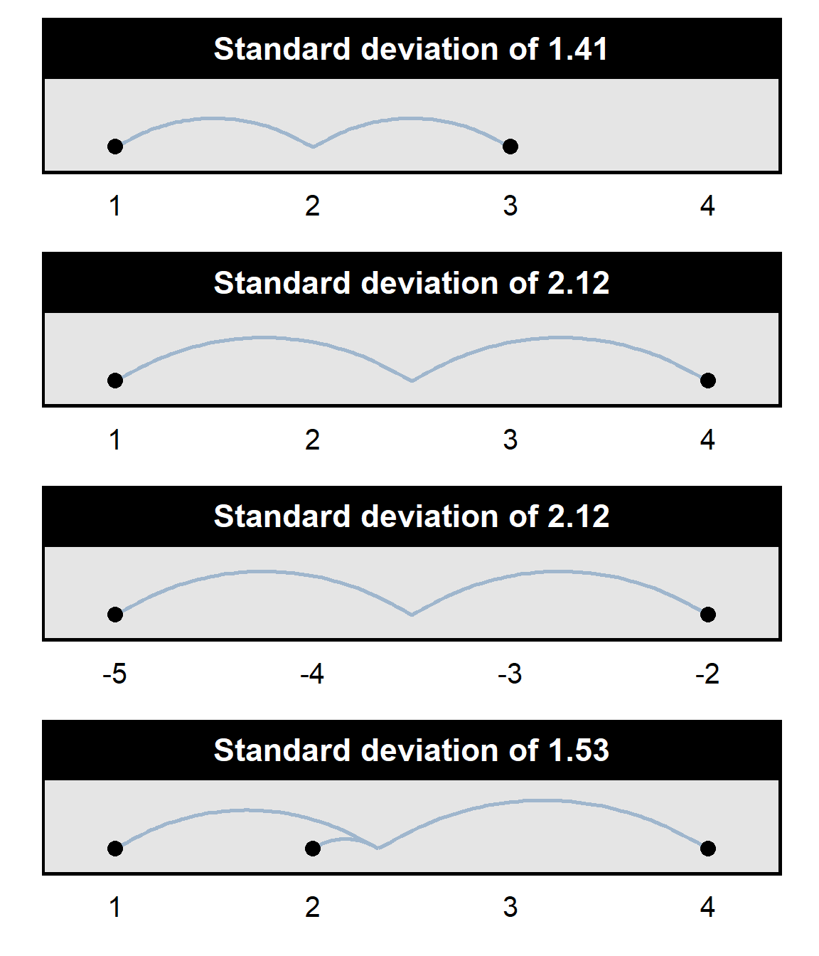
Standard deviations range from 0 (if there is no variation in the set of numbers) to infinity (if there is infinitely large variation in the set of numbers). Students will not need to calculate a standard deviation in this course, but students are expected to correctly respond to items about the fact that standard deviation measures the variation in a set of numbers.
Standard error
A simplified conceptualization of a standard error is as an measure of the precision of an estimate, in which smaller standard errors indicate more precise estimates, all else equal. The standard error depends on the spread of observations but also on sample size: all else equal, a larger spread produces a larger standard error, and, all else equal, a larger sample produces a smaller standard error.
The formula for a standard error depends on what the standard error is for, but the formula for the standard error of the mean is below, with SD indicating the standard deviation and N indicating the sample size:
SE = \(\Large\frac{SD}{\sqrt{N}}\)
So, for the set of whole numbers from 0 to 100, the standard error can be calculated as follows:
The square root of the sample size reflects the fact that the information added with an additional observation decreases as the sample size increases. For instance, adding 10 participants to a sample of 10 will provide more information about the mean of the population than adding 10 participants to a sample of 1,000 would.
For another example, the formula for the standard error for the difference between the means of two independent groups (which we’ll call “Sample 1” and “Sample 2”) is:
\[SE = \sqrt{\frac{\text{Sample 1 std dev}^2}{\text{Sample 1 size}}+\frac{\text{Sample 2 std dev}^2}{\text{Sample 2 size}}}\]
t-statistic
A t-statistic is a point estimate divided by the relevant standard error. For example, the formula for the t-statistic for a difference between the means of two independent groups is:
\[t = \frac{\text{Sample 1 mean - Sample 2 mean}}{\sqrt{\Large\frac{\text{Sample 1 std dev}^2}{\text{Sample 1 size}}+\Large\frac{\text{Sample 2 std dev}^2}{\text{Sample 2 size}}}}\] This formula is merely the estimated difference between the two samples (in the numerator) divided by the standard error for the difference between the means of the two samples.
It’s more complicated that this, but a somewhat close understanding is that, all else equal, the farther a t-statistic is from zero, the more evidence the analysis has provided against the null hypothesis. The complication is that the t-statistic is combined with another measure (degrees of freedom) to calculate the p-value for the analysis.
Sample practice items
Of the following, which best describes what a standard deviation indicates?
- the precision of an estimate
- the strength of an association
- the spread of a set of numbers
- the strength of evidence for the null hypothesis
- the strength of evidence against the null hypothesis
Answer
- the spread of a set of numbers
The standard deviation for the set of numbers {-5,-5,-5} is…
- negative
- zero
- positive
Answer
- zero
The standard deviation for the set of numbers {-5,-6,-7} is…
- negative
- zero
- positive
Answer
- positive
Of the following, which best describes what a standard error indicates?
- the precision of an estimate
- the strength of an association
- the spread of a set of numbers
- the strength of evidence for the null hypothesis
- the strength of evidence against the null hypothesis
Answer
- the precision of an estimate
Which of the following would be the calculation for the standard error of the mean, for a sample that had a mean of M, a standard deviation of SD, and a sample size of N?
- \(\Large\frac{M}{N}\)
- \(\Large\frac{SD}{N}\)
- \(\Large\frac{M}{\sqrt{N}}\)
- \(\Large\frac{SD}{\sqrt{N}}\)
- \(\Large\sqrt{\frac{M * SD}{N}}\)
Answer
- \(\Large\frac{SD}{\sqrt{N}}\)
Based on the formula for a t-statistic for a test of the equality of two means from independent samples, how would an increase in the difference between the Sample 1 mean and the Sample 2 mean change the t-statistic?
- the t-statistic would increase
- the t-statistic would decrease
- the t-statistic would get closer to zero
- the t-statistic would get farther from zero
Answer
- the t-statistic would get farther from zero
Based on the formula for a t-statistic for a test of the equality of two means from independent samples, which of the following t-statistics would be stronger evidence of a difference between two independent samples?
- a t-statistic of 2
- a t-statistic of 5
Answer
- a t-statistic of 5
Based on the formula for a t-statistic for a test of the equality of two means from independent samples, which of the following t-statistics would be stronger evidence of a difference between two independent samples?
- a t-statistic of +2
- a t-statistic of -5
Answer
- a t-statistic of -5
A t-statistic of zero would correspond to which p-value?
- 0
- 0.05
- 0.5
- 0.95
- 1
Answer
- p=1
Which one of the t-statistics below would have the lowest associated p-value, all else equal?
- t = 1
- t = 7
Answer
- t=7
Which one of the t-statistics below would have the lowest associated p-value, all else equal?
- t = -9
- t = 0
- t = 7
Answer
- t = -9
Given a null hypothesis of no difference, increasing the sample size in an experiment will be expected to …, all else equal, if there is a difference between the treatment group and the control group.
- increase the t-statistic
- decrease the t-statistic
- move the t-statistic farther from zero
- move the t-statistic closer to zero
- not change the t-statistic
Answer
- move the t-statistic farther from zero
Suppose that we randomly selected 100 numbers and called those numbers X. We randomly select another 100 numbers and call those 100 numbers Y. We get a p-value for a test of the null hypothesis that X equals Y. We do this over and over again until we get a sufficiently large set of p-values. Which of the following should be the expected mean of these p-values?
- p=0.00
- p=0.05
- p=0.50
- p=0.95
- p=1.00
Answer
- p=0.50
Suppose that we randomly selected 100 numbers and called those numbers X. We randomly select another 100 numbers and call those 100 numbers Y. We get a p-value for a test of the null hypothesis that X equals Y. We do this over and over again until we get a sufficiently large set of p-values. What percentage of these p-values should be less than or equal to p=0.05?
- 0%
- 5%
- 50%
- 95%
- 100%
Answer
- 5%
16.2 Model fit statistics
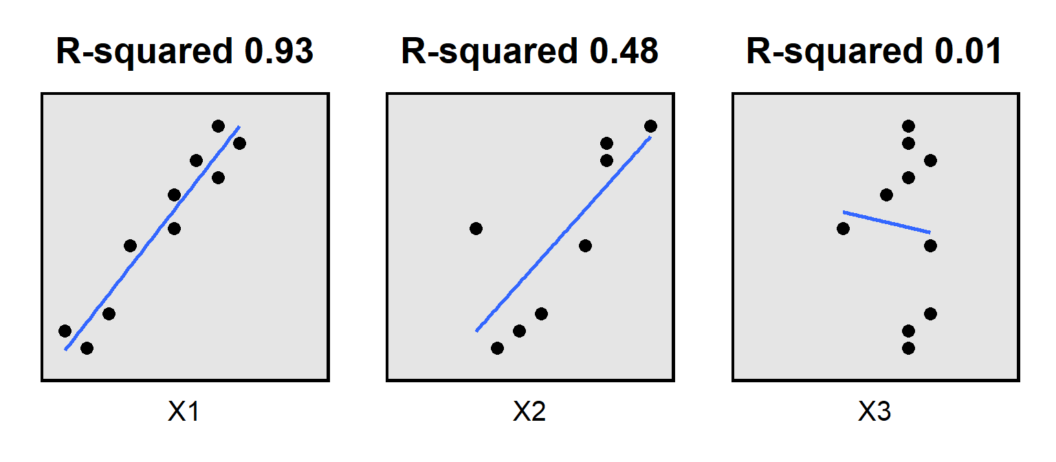
Statistical output often reports model fit statistics about how well the predictors in an analysis predicted the outcome. One such model fit statistic is R-squared, which represents the proportion of the variance in the outcome that the predictors explain. If R-squared is zero, then the predictors explain none of the variance in the outcome; if the R-squared is 1, then the predictors explain all of the variance in the outcome; if the R-squared is between 0 and 1, then the predictors explain some but not all of the variation. For example:
Statistical software can report an adjusted R-squared, for which the R-squared is penalized for each additional predictor in the model. Sometimes an additional predictor is good enough to overcome that penalty, like in the example below, in which X2 was added to X1 when predicting the outcome, raising the adjusted R-squared from 0.413 to 0.917:
reg Y X1
running D:\OneDrive - IL State University\2-teaching\R for teaching\POL497\prof

> ile.do ...

      Source |       SS           df       MS      Number of obs   =        10
-------------+----------------------------------   F(1, 8)         =      7.32
       Model |  95.9875796         1  95.9875796   Prob > F        =    0.0268
    Residual |   104.91242         8  13.1140525   R-squared       =    0.4778
-------------+----------------------------------   Adj R-squared   =    0.4125
       Total |       200.9         9  22.3222222   Root MSE        =    3.6213

------------------------------------------------------------------------------
           Y |      Coef.   Std. Err.      t    P>|t|     [95% Conf. Interval]
-------------+----------------------------------------------------------------
          X1 |      0.874      0.323     2.71   0.027        0.129       1.619
       _cons |      1.057      3.186     0.33   0.748       -6.289       8.404
------------------------------------------------------------------------------
reg Y X2
running D:\OneDrive - IL State University\2-teaching\R for teaching\POL497\prof
> ile.do ...
Source | SS df MS Number of obs = 10
-------------+---------------------------------- F(1, 8) = 95.44
Model | 185.361988 1 185.361988 Prob > F = 0.0000
Residual | 15.5380117 8 1.94225146 R-squared = 0.9227
-------------+---------------------------------- Adj R-squared = 0.9130
Total | 200.9 9 22.3222222 Root MSE = 1.3936
------------------------------------------------------------------------------
Y | Coef. Std. Err. t P>|t| [95% Conf. Interval]
-------------+----------------------------------------------------------------
X2 | 1.646 0.169 9.77 0.000 1.258 2.035
_cons | 0.211 1.011 0.21 0.840 -2.121 2.542
------------------------------------------------------------------------------But sometimes an additional predictor is not good enough to overcome that penalty, like in the example below, in which X3 was added to X1 when predicting the outcome, lowering the adjusted R-squared from 0.413 to 0.392. Note that the penalty applied with R-squared might be enough to make adjusted R-squared negative.
reg Y X1
running D:\OneDrive - IL State University\2-teaching\R for teaching\POL497\prof

> ile.do ...

      Source |       SS           df       MS      Number of obs   =        10
-------------+----------------------------------   F(1, 8)         =      7.32
       Model |  95.9875796         1  95.9875796   Prob > F        =    0.0268
    Residual |   104.91242         8  13.1140525   R-squared       =    0.4778
-------------+----------------------------------   Adj R-squared   =    0.4125
       Total |       200.9         9  22.3222222   Root MSE        =    3.6213

------------------------------------------------------------------------------
           Y |      Coef.   Std. Err.      t    P>|t|     [95% Conf. Interval]
-------------+----------------------------------------------------------------
          X1 |      0.874      0.323     2.71   0.027        0.129       1.619
       _cons |      1.057      3.186     0.33   0.748       -6.289       8.404
------------------------------------------------------------------------------
reg Y X3
running D:\OneDrive - IL State University\2-teaching\R for teaching\POL497\prof
> ile.do ...
Source | SS df MS Number of obs = 10
-------------+---------------------------------- F(1, 8) = 0.05
Model | 1.17906977 1 1.17906977 Prob > F = 0.8334
Residual | 199.72093 8 24.9651163 R-squared = 0.0059
-------------+---------------------------------- Adj R-squared = -0.1184
Total | 200.9 9 22.3222222 Root MSE = 4.9965
------------------------------------------------------------------------------
Y | Coef. Std. Err. t P>|t| [95% Conf. Interval]
-------------+----------------------------------------------------------------
X3 | -0.302 1.391 -0.22 0.833 -3.510 2.906
_cons | 11.488 11.103 1.03 0.331 -14.115 37.092
------------------------------------------------------------------------------Remember that residuals are the differences between the observed values and the predicted values. R-squared is calculated based on minimizing the sum of the squared residuals, but that calculation is not appropriate for types of regression that are not based on minimizing the sum of the squared residuals. So output for other types of regressions might report a pseudo R2 goodness-of-fit statistic, like for the logit regression below:
logit DICHOTOMOUS_OUTCOME PREDICTOR
running D:\OneDrive - IL State University\2-teaching\R for teaching\POL497\prof

> ile.do ...


Iteration 0:   log likelihood = -6.9314718
Iteration 1:   log likelihood = -5.5893843
Iteration 2:   log likelihood =  -5.586334
Iteration 3:   log likelihood = -5.5863321
Iteration 4:   log likelihood = -5.5863321

Logistic regression                             Number of obs     =         10
                                                LR chi2(1)        =       2.69
                                                Prob > chi2       =     0.1010
Log likelihood = -5.5863321                     Pseudo R2         =     0.1941

------------------------------------------------------------------------------
DICHOTOMOU~E |      Coef.   Std. Err.      z    P>|z|     [95% Conf. Interval]
-------------+----------------------------------------------------------------
   PREDICTOR |      0.452      0.313     1.44   0.149       -0.162       1.067
       _cons |     -2.420      1.852    -1.31   0.191       -6.049       1.210
------------------------------------------------------------------------------
Note that a relatively small R-squared for a regression does not necessarily indicate that the regression model has been poorly designed. Some outcomes are more difficult to predict, which can be reflected in a relatively small R-squared.
Sample practice items
Of the following, which best describes what R-squared indicates for a linear regression?
- the sum of the squared residuals
- the proportion of the variance explained
- the strength of evidence against the null hypothesis
- the percentage of outcomes that are correctly predicted
Answer
- the proportion of the variance explained
Adding a predictor that correlates with the outcome variable independently of the predictors already present in a model ___ cause R-squared to increase.
- will
- might
- will not
Answer
- will
Adding a predictor that correlates with the outcome variable independently of the predictors already present in a model ___ cause adjusted R-squared to increase.
- will
- might
- will not
Answer
- might
Can R-squared be negative?
- Yes
- No
Answer
- No
Can adjusted R-squared be negative?
- Yes
- No
Answer
- Yes
16.3 Clustering observations
Sometimes a dataset has observations that are not independent of each other. For example, there are 1,883 observations in the data for Zigerell 2014 “Senator Opposition to Supreme Court Nominations: Reference Dependence on the Departing Justice”, but these 1,883 observations are from only 323 different senators, because some senators voted on more than one U.S. Supreme Court nomination in the dataset; for example, Ted Kennedy voted on all 19 nominations in the dataset, so 19 of the 1,883 observations are for Ted Kennedy. Nineteen observations from Ted Kennedy do not provide the same information about senator voting decisions as would be provided if the same observations had been provided by nineteen different senators voting once. So, to account for this, our analyses should cluster observations.
Let’s run an analysis predicting senator opposition using robust standard errors but without clustering:
logit SENOPP NOMQUAL DIFPARTY, robust nolog
running D:\OneDrive - IL State University\2-teaching\R for teaching\POL497\prof

> ile.do ...


Logistic regression                             Number of obs     =      1,883
                                                Wald chi2(2)      =     316.70
                                                Prob > chi2       =     0.0000
Log pseudolikelihood = -718.27703               Pseudo R2         =     0.2721

------------------------------------------------------------------------------
             |               Robust
      SENOPP |      Coef.   Std. Err.      z    P>|z|     [95% Conf. Interval]
-------------+----------------------------------------------------------------
     NOMQUAL |     -3.921      0.250   -15.71   0.000       -4.410      -3.432
    DIFPARTY |      2.348      0.170    13.82   0.000        2.015       2.681
       _cons |     -0.050      0.190    -0.27   0.791       -0.422       0.322
------------------------------------------------------------------------------
Remember that the t-statistic (also called a t-value) can be considered a measure of evidence in which a t-statistic of 0 indicates that an analysis provided no evidence against the null hypothesis and, the farther the t-statistic is from 0, the more evidence that the analysis provided evidence against the null hypothesis, all else equal. For the above regression, using robust standard errors but without clustering, the t-value is -15.71 for the measure of nominee qualifications (NOMQUAL) and is 13.82 for the measure of whether the senator has a different political party than the president does (DIFFPARTY).
The regression below uses robust standard errors and clusters observations by senator (SENATORID), so that the analysis accounts for the fact that some senators appear multiple times in the data so that these observations are not independent of each other. The coefficient estimates did not change, but the inferential statistics did change: the t-values got smaller, the p-values got farther from zero (but still rounded to 0.00 in this output), and the confidence intervals got wider, all of which indicate less evidence against the null hypothesis.
logit SENOPP NOMQUAL DIFPARTY, cluster(SENATORID) nolog
running D:\OneDrive - IL State University\2-teaching\R for teaching\POL497\prof

> ile.do ...


Logistic regression                             Number of obs     =      1,883
                                                Wald chi2(2)      =     198.66
                                                Prob > chi2       =     0.0000
Log pseudolikelihood = -718.27703               Pseudo R2         =     0.2721

                            (Std. Err. adjusted for 323 clusters in SENATORID)
------------------------------------------------------------------------------
             |               Robust
      SENOPP |      Coef.   Std. Err.      z    P>|z|     [95% Conf. Interval]
-------------+----------------------------------------------------------------
     NOMQUAL |     -3.921      0.281   -13.95   0.000       -4.472      -3.370
    DIFPARTY |      2.348      0.250     9.41   0.000        1.859       2.837
       _cons |     -0.050      0.204    -0.25   0.805       -0.450       0.349
------------------------------------------------------------------------------
Clustering observations often reduces the amount of evidence that an analysis provides against the null hypothesis. For example, observing Ted Kennedy vote 19 times provided more information about Ted Kennedy than would have been provided by observing Ted Kennedy vote only one time, but observing Ted Kennedy vote 19 times did not provide as much information about senator voting as would have been provided by observing 19 different senators each vote once.
But clustering observations does not always reduce the amount of evidence that an analysis provides against the null hypothesis. For instance, the hypothetical data below has four raters (IDs A through D) who each provided three ratings (RATING) for nominees that had a measured nominee quality of NOMQUAL.
# A tibble: 12 × 3
   ID    NOMQUAL RATING
   <chr>   <dbl>  <dbl>
 1 A          50     65
 2 A          60     67
 3 A          70     68
 4 B          50     61
 5 B          60     62
 6 B          70     64
 7 C          50     56
 8 C          60     57
 9 C          70     59
10 D          50     52
11 D          60     52
12 D          70     53
In the regression below, without clustering, the p-value for NOMQUAL is p=0.555.
reg RATING NOMQUAL, robust
running D:\OneDrive - IL State University\2-teaching\R for teaching\POL497\prof

> ile.do ...


Linear regression                               Number of obs     =         12
                                                F(1, 10)          =       0.37
                                                Prob > F          =     0.5547
                                                R-squared         =     0.0347
                                                Root MSE          =     5.9006

------------------------------------------------------------------------------
             |               Robust
      RATING |      Coef.   Std. Err.      t    P>|t|     [95% Conf. Interval]
-------------+----------------------------------------------------------------
     NOMQUAL |      0.125      0.205     0.61   0.555       -0.331       0.581
       _cons |     52.167     12.211     4.27   0.002       24.958      79.375
------------------------------------------------------------------------------
But with clustering the p-value is p=0.018, which provides much more evidence against the null hypothesis that NOMQUAL is zero, compared to the evidence that the analysis without clustering provided.
reg RATING NOMQUAL, cluster(ID)
running D:\OneDrive - IL State University\2-teaching\R for teaching\POL497\prof
> ile.do ...
Linear regression Number of obs = 12
F(1, 3) = 22.73
Prob > F = 0.0175
R-squared = 0.0347
Root MSE = 5.9006
(Std. Err. adjusted for 4 clusters in ID)
------------------------------------------------------------------------------
| Robust
RATING | Coef. Std. Err. t P>|t| [95% Conf. Interval]
-------------+----------------------------------------------------------------
NOMQUAL | 0.125 0.026 4.77 0.018 0.042 0.208
_cons | 52.167 2.232 23.38 0.000 45.064 59.269
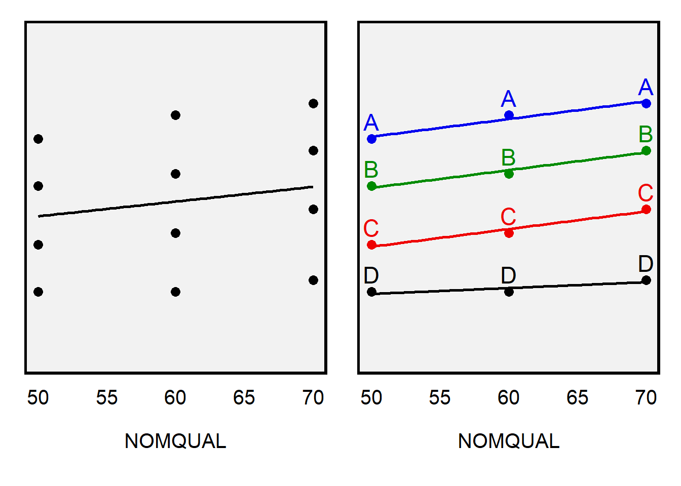
------------------------------------------------------------------------------The plot below explains how the clustering led to a lower p-value. The left panel presents the data as used in the regression without clustering: 12 independent observations that have a slight positive association between NOMQUAL and RATING. But the right panel indicates that incorporating information about which observations are from which raters suggests a stronger association between NOMQUAL and RATING, with a positive association for all four raters. The consistency in the right panel provides more evidence that the association is not zero, compared to merely treating the 12 points as independent observations.
Sample practice items
A regression should cluster standard errors if…
- the observations are not independent of each other
- the sample characteristics do not match the population characteristics
- the outcome variable has an outlier
- a test indicated the presence of heteroskedasticity
Answer
- the observations are not independent of each other
Compared to an analysis that did not cluster observations, can an analysis that clustered observations produce p-values that are closer to 1 (and thus indicate weaker evidence against the null hypothesis)?
- Yes
- No
Answer
- Yes
Compared to an analysis that did not cluster observations, can an analysis that clustered observations produce p-values that are closer to 0 (and thus indicate stronger evidence against the null hypothesis)?
- Yes
- No
Answer
- Yes
16.4 Factor analysis
Factor analysis is a method that researchers can use to assess whether multiple measures capture the same phenomenon well enough to justify combining the measures into a single measure. The goal for a variable is to arrange cases on a scale as accurately and as precisely as possible, to address our research question. Multiple items combined into one measure can help us better arrange our cases.
Consider these four items from the ANES 2016 Time Series Study.
Should the news media pay more attention to discrimination against women, less attention, or the same amount of attention they have been paying lately?
When women demand equality these days, how often are they actually seeking special favors?
Do you think it is easier, harder, or neither easier nor harder for mothers who work outside the home to establish a warm and secure relationship with their children than it is for mothers who stay at home?
Do you think it is better, worse, or makes no difference for the family as a whole if the man works outside the home and the woman takes care of the home and family?
These items had follow-up items that measured these phenomena in more detail, with measures having five or seven points. For example, response options for the third item were: A great deal easier, Somewhat easier, Slightly easier, Neither easier nor harder, Slightly harder, Somewhat harder, and A great deal harder. Let’s illustrate how factor analysis can be used to assess whether these items capture a general “gender attitudes” phenomenon. First, let’s run the “factor” command in stata, with the “pcf” option to identify principal components.
factor ATTN DEMAND BOND CARE, pcf
running D:\OneDrive - IL State University\2-teaching\R for teaching\POL497\prof

> ile.do ...


(obs=3,528)

Factor analysis/correlation                      Number of obs    =      3,528
    Method: principal-component factors          Retained factors =          2
    Rotation: (unrotated)                        Number of params =          6

    --------------------------------------------------------------------------
         Factor  |   Eigenvalue   Difference        Proportion   Cumulative
    -------------+------------------------------------------------------------
        Factor1  |      1.50070      0.32916            0.3752       0.3752
        Factor2  |      1.17154      0.44839            0.2929       0.6681
        Factor3  |      0.72315      0.11853            0.1808       0.8488
        Factor4  |      0.60462            .            0.1512       1.0000
    --------------------------------------------------------------------------
    LR test: independent vs. saturated:  chi2(6)  =  927.48 Prob>chi2 = 0.0000

Factor loadings (pattern matrix) and unique variances

    -------------------------------------------------
        Variable |  Factor1   Factor2 |   Uniqueness
    -------------+--------------------+--------------
            ATTN |  -0.6163   -0.5768 |      0.2874
          DEMAND |   0.7089    0.3805 |      0.3527
            BOND |  -0.4809    0.6829 |      0.3024
            CARE |   0.6221   -0.4772 |      0.3853
    -------------------------------------------------
This factor analysis method has identified two factors. The “rotate” command (with output below) lets us better assess whether measures loaded onto which factor. Numbers farther from zero indicate stronger loading onto that factor. So, for example, ATTN and DEMAND loaded onto the first factor, and BOND and CARE loaded onto the second factor. ATTN and DEMAND have opposite signs, because the patterns are in the opposite direction: the highest value for ATTN indicates that the respondent thinks that a great deal less attention should be paid to discrimination against women, and the highest value for DEMAND indicates that the respondent thinks that women demanding equality are never seeking special favors.
rotate
running D:\OneDrive - IL State University\2-teaching\R for teaching\POL497\prof

> ile.do ...


Factor analysis/correlation                      Number of obs    =      3,528
    Method: principal-component factors          Retained factors =          2
    Rotation: orthogonal varimax (Kaiser off)    Number of params =          6

    --------------------------------------------------------------------------
         Factor  |     Variance   Difference        Proportion   Cumulative
    -------------+------------------------------------------------------------
        Factor1  |      1.36793      0.06362            0.3420       0.3420
        Factor2  |      1.30431            .            0.3261       0.6681
    --------------------------------------------------------------------------
    LR test: independent vs. saturated:  chi2(6)  =  927.48 Prob>chi2 = 0.0000

Rotated factor loadings (pattern matrix) and unique variances

    -------------------------------------------------
        Variable |  Factor1   Factor2 |   Uniqueness
    -------------+--------------------+--------------
            ATTN |  -0.8424    0.0541 |      0.2874
          DEMAND |   0.7892    0.1563 |      0.3527
            BOND |   0.0622   -0.8329 |      0.3024
            CARE |   0.1775    0.7637 |      0.3853
    -------------------------------------------------

Factor rotation matrix

    --------------------------------
                 | Factor1  Factor2
    -------------+------------------
         Factor1 |  0.7724
         Factor2 |  0.6351  -0.7724
    --------------------------------
This “rotate” output suggests that we should consider not combining these four items into a single measure of gender attitudes, because the ATTN and FAVORS measures loaded onto a different factor than the BOND and CARE measures did. Factor analysis doesn’t tell us what these factors measure, but we can usually figure that out. In this case, ATTN and FAVORS might capture attitudes about women, and BOND and CARE might capture attitudes about traditional gender roles.
Let’s try another example, with four measures that are commonly used to measure a concept called “racial resentment”:
- Irish, Italians, Jewish and many other minorities overcame prejudice and worked their way up. Blacks should do the same without any special favors.
- Generations of slavery and discrimination have created conditions that make it difficult for blacks to work their way out of the lower class.
- Over the past few years, blacks have gotten less than they deserve.
- It’s really a matter of some people not trying hard enough; if blacks would only try harder they could be just as well off as whites.
factor FAVORS SLAVERY DESERVE TRY, pcf
running D:\OneDrive - IL State University\2-teaching\R for teaching\POL497\prof

> ile.do ...


(obs=3,612)

Factor analysis/correlation                      Number of obs    =      3,612
    Method: principal-component factors          Retained factors =          1
    Rotation: (unrotated)                        Number of params =          4

    --------------------------------------------------------------------------
         Factor  |   Eigenvalue   Difference        Proportion   Cumulative
    -------------+------------------------------------------------------------
        Factor1  |      2.73703      2.12151            0.6843       0.6843
        Factor2  |      0.61552      0.28304            0.1539       0.8381
        Factor3  |      0.33248      0.01752            0.0831       0.9213
        Factor4  |      0.31497            .            0.0787       1.0000
    --------------------------------------------------------------------------
    LR test: independent vs. saturated:  chi2(6)  = 6262.60 Prob>chi2 = 0.0000

Factor loadings (pattern matrix) and unique variances

    ---------------------------------------
        Variable |  Factor1 |   Uniqueness
    -------------+----------+--------------
          FAVORS |  -0.8328 |      0.3064
         SLAVERY |   0.8162 |      0.3339
         DESERVE |   0.8418 |      0.2914
             TRY |  -0.8177 |      0.3313
    ---------------------------------------
rotate
running D:\OneDrive - IL State University\2-teaching\R for teaching\POL497\prof
> ile.do ...
Factor analysis/correlation Number of obs = 3,612
Method: principal-component factors Retained factors = 1
Rotation: orthogonal varimax (Kaiser off) Number of params = 4
--------------------------------------------------------------------------
Factor | Variance Difference Proportion Cumulative
-------------+------------------------------------------------------------
Factor1 | 2.73703 . 0.6843 0.6843
--------------------------------------------------------------------------
LR test: independent vs. saturated: chi2(6) = 6262.60 Prob>chi2 = 0.0000
Rotated factor loadings (pattern matrix) and unique variances
---------------------------------------
Variable | Factor1 | Uniqueness
-------------+----------+--------------
FAVORS | -0.8328 | 0.3064
SLAVERY | 0.8162 | 0.3339
DESERVE | 0.8418 | 0.2914
TRY | -0.8177 | 0.3313
---------------------------------------
Factor rotation matrix
-----------------------
| Factor1
-------------+---------
Factor1 | 1.0000
-----------------------In this case, the four measures loaded onto the same factor, so that we can be reasonably confident that these measures are capturing something similar enough to be combined into one measure. Factor analysis doesn’t tell us what these factors measure, and it’s not clear from this analysis whether the factor should be interpreted as attitudes about Blacks or attitudes about racial inequality or something such as perceptions about the reasons for Black/White inequality.
If one factor is present, the “predict” command run after a “factor” command or a “rotate” command will generate a variable that has one number for each respondent who has sufficient data.
predict RRfactor
running D:\OneDrive - IL State University\2-teaching\R for teaching\POL497\prof

> ile.do ...


(regression scoring assumed)

Scoring coefficients (method = regression; based on varimax rotated factors)

    ------------------------
        Variable |  Factor1
    -------------+----------
          FAVORS | -0.30428
         SLAVERY |  0.29819
         DESERVE |  0.30756
             TRY | -0.29877
    ------------------------
sum RRfactor
running D:\OneDrive - IL State University\2-teaching\R for teaching\POL497\prof
> ile.do ...
Variable | Obs Mean Std. Dev. Min Max
-------------+---------------------------------------------------------
RRfactor | 3,612 -1.13e-09 1 -1.930586 1.590886In this case, the variable from the “predict” command is pretty similar to merely summing the four items, as indicated below. But sometimes that isn’t true, especially if the measures have different scale lengths, such as one measure being on a scale from 1 through 5 and another measure being on a scale of 1 through 7.
gen RRsum = -FAVORS + SLAVERY + DESERVE -TRY
running D:\OneDrive - IL State University\2-teaching\R for teaching\POL497\prof

> ile.do ...


(658 missing values generated)
sum RRfactor RRsum
running D:\OneDrive - IL State University\2-teaching\R for teaching\POL497\prof
> ile.do ...
Variable | Obs Mean Std. Dev. Min Max
-------------+---------------------------------------------------------
RRfactor | 3,612 -1.13e-09 1 -1.930586 1.590886
RRsum | 3,612 .7574751 4.547163 -8 8pwcorr RRfactor RRsum
running D:\OneDrive - IL State University\2-teaching\R for teaching\POL497\prof
> ile.do ...
| RRfactor RRsum
-------------+------------------
RRfactor | 1.0000
RRsum | 0.9999 1.0000 One of the benefits of combining measures is that the combined measure should better predict outcomes. Check below, in which a seven-point PARTY variable that ranges from 1 for Strong Democrat to 7 for Strong Republican correlates more strongly with the the combined RRfactor than with any of the four individual racial resentment items.
pwcorr PARTY FAVORS SLAVERY DESERVE TRY RRfactor
running D:\OneDrive - IL State University\2-teaching\R for teaching\POL497\prof

> ile.do ...

             |    PARTY   FAVORS  SLAVERY  DESERVE      TRY RRfactor
-------------+------------------------------------------------------
       PARTY |   1.0000
      FAVORS |  -0.4412   1.0000
     SLAVERY |   0.4031  -0.5205   1.0000
     DESERVE |   0.4428  -0.5638   0.6793   1.0000
         TRY |  -0.3993   0.6685  -0.5024  -0.5339   1.0000
    RRfactor |   0.5104  -0.8328   0.8162   0.8418  -0.8177   1.0000
For another illustration of how the combined RRfactor is useful, check how relatively few respondents fall into an extreme category for the RRfactor measure compared to the other measures:
tab1 FAVORS SLAVERY DESERVE TRY RRfactor
running D:\OneDrive - IL State University\2-teaching\R for teaching\POL497\prof
> ile.do ...
-> tabulation of FAVORS
POST: Agree/disagree: blacks shd work |
way up w/o special favors | Freq. Percent Cum.
----------------------------------------+-----------------------------------
1. Agree strongly | 1,110 30.59 30.59
2. Agree somewhat | 912 25.13 55.72
3. Neither agree nor disagree | 647 17.83 73.55
4. Disagree somewhat | 474 13.06 86.61
5. Disagree strongly | 486 13.39 100.00
----------------------------------------+-----------------------------------
Total | 3,629 100.00
-> tabulation of SLAVERY
POST: Agree/disagree: past slavery make |
more diff for blacks | Freq. Percent Cum.
----------------------------------------+-----------------------------------
1. Agree strongly | 645 17.75 17.75
2. Agree somewhat | 986 27.13 44.88
3. Neither agree nor disagree | 512 14.09 58.97
4. Disagree somewhat | 706 19.43 78.40
5. Disagree strongly | 785 21.60 100.00
----------------------------------------+-----------------------------------
Total | 3,634 100.00
-> tabulation of DESERVE
POST: Agree/disagree: blacks have |
gotten less than deserve | Freq. Percent Cum.
----------------------------------------+-----------------------------------
1. Agree strongly | 410 11.29 11.29
2. Agree somewhat | 695 19.15 30.44
3. Neither agree nor disagree | 936 25.79 56.23
4. Disagree somewhat | 711 19.59 75.81
5. Disagree strongly | 878 24.19 100.00
----------------------------------------+-----------------------------------
Total | 3,630 100.00
-> tabulation of TRY
POST: Agree/disagree: blacks must try |
harder to get ahead | Freq. Percent Cum.
----------------------------------------+-----------------------------------
1. Agree strongly | 629 17.35 17.35
2. Agree somewhat | 871 24.02 41.37
3. Neither agree nor disagree | 785 21.65 63.02
4. Disagree somewhat | 668 18.42 81.44
5. Disagree strongly | 673 18.56 100.00
----------------------------------------+-----------------------------------
Total | 3,626 100.00
-> tabulation of RRfactor
Scores for |
factor 1 | Freq. Percent Cum.
------------+-----------------------------------
-1.930586 | 186 5.15 5.15
-1.721916 | 19 0.53 5.68
-1.711616 | 13 0.36 6.04
-1.711324 | 22 0.61 6.64
-1.697118 | 70 1.94 8.58
-1.513247 | 2 0.06 8.64
-1.502947 | 4 0.11 8.75
-1.502655 | 7 0.19 8.94
-1.492647 | 1 0.03 8.97
-1.492355 | 2 0.06 9.03
-1.492062 | 6 0.17 9.19
-1.488449 | 22 0.61 9.80
-1.478149 | 13 0.36 10.16
-1.477856 | 33 0.91 11.07
-1.46365 | 20 0.55 11.63
-1.283685 | 3 0.08 11.71
-1.283393 | 2 0.06 11.77
-1.273678 | 3 0.08 11.85
-1.273385 | 2 0.06 11.90
-1.2728 | 8 0.22 12.13
-1.269479 | 15 0.42 12.54
-1.269187 | 42 1.16 13.70
-1.258887 | 15 0.42 14.12
-1.258595 | 6 0.17 14.29
-1.254981 | 11 0.30 14.59
-1.244681 | 2 0.06 14.65
-1.244389 | 6 0.17 14.81
-1.230183 | 4 0.11 14.92
-1.095909 | 1 0.03 14.95
-1.085316 | 1 0.03 14.98
-1.074724 | 2 0.06 15.03
-1.07111 | 2 0.06 15.09
-1.065008 | 1 0.03 15.12
-1.064716 | 2 0.06 15.17
-1.064423 | 1 0.03 15.20
-1.064131 | 2 0.06 15.25
-1.06081 | 1 0.03 15.28
-1.060518 | 5 0.14 15.42
-1.054708 | 5 0.14 15.56
-1.054416 | 1 0.03 15.59
-1.054123 | 2 0.06 15.64
-1.053831 | 6 0.17 15.81
-1.053539 | 9 0.25 16.06
-1.05051 | 2 0.06 16.11
-1.050218 | 71 1.97 18.08
-1.049925 | 8 0.22 18.30
-1.046312 | 3 0.08 18.38
-1.04021 | 3 0.08 18.47
-1.039918 | 2 0.06 18.52
-1.039625 | 7 0.19 18.72
-1.039333 | 4 0.11 18.83
-1.036012 | 7 0.19 19.02
-1.03572 | 18 0.50 19.52
-1.025712 | 3 0.08 19.60
-1.025419 | 9 0.25 19.85
-1.025127 | 2 0.06 19.91
-1.021514 | 4 0.11 20.02
-1.011214 | 1 0.03 20.04
-1.010921 | 1 0.03 20.07
-.9967154 | 2 0.06 20.13
-.8769392 | 2 0.06 20.18
-.8766469 | 1 0.03 20.21
-.8663468 | 1 0.03 20.24
-.8624411 | 2 0.06 20.29
-.852141 | 2 0.06 20.35
-.8518485 | 2 0.06 20.40
-.8454542 | 1 0.03 20.43
-.8451617 | 4 0.11 20.54
-.8418409 | 1 0.03 20.57
-.8415484 | 4 0.11 20.68
-.8412561 | 2 0.06 20.74
-.8376428 | 3 0.08 20.82
-.8354464 | 2 0.06 20.87
-.8351541 | 3 0.08 20.96
-.8348616 | 3 0.08 21.04
-.8345692 | 2 0.06 21.10
-.8312483 | 9 0.25 21.35
-.8309559 | 30 0.83 22.18
-.8306636 | 9 0.25 22.43
-.8270503 | 2 0.06 22.48
-.8212406 | 1 0.03 22.51
-.8209482 | 3 0.08 22.59
-.8206558 | 2 0.06 22.65
-.8203635 | 6 0.17 22.81
-.820071 | 2 0.06 22.87
-.8170425 | 1 0.03 22.90
-.8167502 | 44 1.22 24.11
-.8164577 | 6 0.17 24.28
-.8064501 | 1 0.03 24.31
-.8061576 | 4 0.11 24.42
-.8058652 | 1 0.03 24.45
-.8022519 | 5 0.14 24.58
-.7919518 | 2 0.06 24.64
-.7777461 | 1 0.03 24.67
-.6576775 | 1 0.03 24.70
-.647085 | 1 0.03 24.72
-.6434717 | 1 0.03 24.75
-.6373697 | 2 0.06 24.81
-.6367849 | 1 0.03 24.83
-.6364925 | 1 0.03 24.86
-.6328792 | 8 0.22 25.08
-.6325868 | 2 0.06 25.14
-.6289735 | 2 0.06 25.19
-.6264848 | 2 0.06 25.25
-.6261924 | 2 0.06 25.30
-.6259 | 1 0.03 25.33
-.6222867 | 6 0.17 25.50
-.618381 | 3 0.08 25.58
-.6161847 | 1 0.03 25.61
-.6158923 | 9 0.25 25.86
-.6155999 | 1 0.03 25.89
-.6125714 | 1 0.03 25.91
-.612279 | 9 0.25 26.16
-.6119866 | 12 0.33 26.50
-.6116942 | 29 0.80 27.30
-.6114018 | 1 0.03 27.33
-.6083733 | 1 0.03 27.35
-.6080809 | 4 0.11 27.46
-.6077885 | 5 0.14 27.60
-.6041752 | 1 0.03 27.63
-.6019789 | 1 0.03 27.66
-.6016865 | 4 0.11 27.77
-.6013941 | 1 0.03 27.80
-.6011017 | 4 0.11 27.91
-.5980732 | 1 0.03 27.93
-.5977808 | 15 0.42 28.35
-.5974884 | 29 0.80 29.15
-.597196 | 4 0.11 29.26
-.5938751 | 1 0.03 29.29
-.5877731 | 1 0.03 29.32
-.5874807 | 1 0.03 29.35
-.5868959 | 6 0.17 29.51
-.5866035 | 1 0.03 29.54
-.5832826 | 14 0.39 29.93
-.5829902 | 4 0.11 30.04
-.5687844 | 1 0.03 30.07
-.4387082 | 1 0.03 30.09
-.4281156 | 2 0.06 30.15
-.4278232 | 2 0.06 30.20
-.4245023 | 1 0.03 30.23
-.42421 | 1 0.03 30.26
-.4239176 | 1 0.03 30.29
-.4139099 | 2 0.06 30.34
-.4136175 | 6 0.17 30.51
-.4133251 | 1 0.03 30.54
-.4100042 | 1 0.03 30.56
-.4075154 | 1 0.03 30.59
-.407223 | 2 0.06 30.65
-.4036098 | 1 0.03 30.68
-.4033174 | 10 0.28 30.95
-.4030249 | 7 0.19 31.15
-.3994116 | 9 0.25 31.40
-.3991193 | 3 0.08 31.48
-.3969229 | 4 0.11 31.59
-.3966305 | 4 0.11 31.70
-.395506 | 1 0.03 31.73
-.3933096 | 1 0.03 31.76
-.3930172 | 6 0.17 31.92
-.3927248 | 9 0.25 32.17
-.3924325 | 3 0.08 32.25
-.3894039 | 1 0.03 32.28
-.3891115 | 6 0.17 32.45
-.3888192 | 10 0.28 32.72
-.3885268 | 2 0.06 32.78
-.3849135 | 5 0.14 32.92
-.3824247 | 5 0.14 33.06
-.3821324 | 2 0.06 33.11
-.3788114 | 3 0.08 33.19
-.3785191 | 30 0.83 34.03
-.3782267 | 28 0.78 34.80
-.3779342 | 2 0.06 34.86
-.3749058 | 2 0.06 34.91
-.3746133 | 4 0.11 35.02
-.374321 | 1 0.03 35.05
-.3707077 | 3 0.08 35.13
-.3682189 | 1 0.03 35.16
-.3679265 | 6 0.17 35.33
-.3676341 | 5 0.14 35.47
-.3646056 | 1 0.03 35.49
-.3643132 | 8 0.22 35.71
-.3640209 | 14 0.39 36.10
-.3637285 | 5 0.14 36.24
-.3540131 | 1 0.03 36.27
-.3537208 | 1 0.03 36.30
-.3534284 | 1 0.03 36.32
-.3498151 | 1 0.03 36.35
-.2200312 | 1 0.03 36.38
-.2194464 | 1 0.03 36.41
-.2046558 | 1 0.03 36.43
-.1985538 | 3 0.08 36.52
-.1949405 | 2 0.06 36.57
-.1946481 | 5 0.14 36.71
-.1943557 | 6 0.17 36.88
-.1940633 | 1 0.03 36.90
-.19045 | 2 0.06 36.96
-.1882537 | 2 0.06 37.02
-.1879613 | 1 0.03 37.04
-.184348 | 4 0.11 37.15
-.1840556 | 6 0.17 37.32
-.1837632 | 1 0.03 37.35
-.1804423 | 2 0.06 37.40
-.1801499 | 12 0.33 37.74
-.1776612 | 18 0.50 38.23
-.1765366 | 3 0.08 38.32
-.1740479 | 3 0.08 38.40
-.1737555 | 42 1.16 39.56
-.1734631 | 2 0.06 39.62
-.1701422 | 3 0.08 39.70
-.1698498 | 171 4.73 44.44
-.1695574 | 4 0.11 44.55
-.1662365 | 1 0.03 44.57
-.1659441 | 11 0.30 44.88
-.1656517 | 2 0.06 44.93
-.1634554 | 1 0.03 44.96
-.163163 | 6 0.17 45.13
-.1620384 | 11 0.30 45.43
-.1598421 | 2 0.06 45.49
-.1595497 | 7 0.19 45.68
-.1592573 | 24 0.66 46.35
-.1589649 | 3 0.08 46.43
-.155644 | 1 0.03 46.46
-.1553516 | 5 0.14 46.59
-.1517383 | 1 0.03 46.62
-.1489572 | 1 0.03 46.65
-.1486648 | 5 0.14 46.79
-.1453439 | 4 0.11 46.90
-.1450515 | 10 0.28 47.18
-.1447591 | 15 0.42 47.59
-.1341666 | 1 0.03 47.62
-.1311381 | 1 0.03 47.65
-.1308457 | 2 0.06 47.70
-.1305533 | 2 0.06 47.76
-.1302609 | 1 0.03 47.79
-.1199608 | 2 0.06 47.84
-.1196684 | 2 0.06 47.90
.0143135 | 1 0.03 47.92
.020708 | 1 0.03 47.95
.0246136 | 7 0.19 48.15
.0285193 | 3 0.08 48.23
.0288117 | 2 0.06 48.28
.0310081 | 1 0.03 48.31
.0349138 | 2 0.06 48.37
.0352061 | 2 0.06 48.42
.038527 | 2 0.06 48.48
.0388194 | 24 0.66 49.14
.0391118 | 10 0.28 49.42
.0394042 | 1 0.03 49.45
.0430175 | 2 0.06 49.50
.0452139 | 5 0.14 49.64
.0455063 | 17 0.47 50.11
.0491196 | 6 0.17 50.28
.0494119 | 21 0.58 50.86
.0497043 | 1 0.03 50.89
.0527328 | 1 0.03 50.91
.0530252 | 3 0.08 51.00
.0533176 | 8 0.22 51.22
.05361 | 5 0.14 51.36
.0558064 | 9 0.25 51.61
.0572233 | 2 0.06 51.66
.0597121 | 30 0.83 52.49
.0600044 | 10 0.28 52.77
.0633253 | 2 0.06 52.82
.0636177 | 11 0.30 53.13
.0639101 | 5 0.14 53.27
.0642025 | 1 0.03 53.29
.0675234 | 2 0.06 53.35
.0678158 | 1 0.03 53.38
.0700122 | 2 0.06 53.43
.0703046 | 6 0.17 53.60
.0736255 | 1 0.03 53.63
.0739179 | 7 0.19 53.82
.0742102 | 18 0.50 54.32
.0745026 | 8 0.22 54.54
.0778235 | 1 0.03 54.57
.0781159 | 4 0.11 54.68
.0784083 | 2 0.06 54.73
.0845103 | 2 0.06 54.79
.0848027 | 1 0.03 54.82
.088416 | 2 0.06 54.87
.0887084 | 3 0.08 54.96
.0890008 | 2 0.06 55.01
.2187847 | 1 0.03 55.04
.2335753 | 1 0.03 55.07
.2396773 | 1 0.03 55.09
.243583 | 4 0.11 55.20
.2438754 | 3 0.08 55.29
.2474887 | 3 0.08 55.37
.2477811 | 5 0.14 55.51
.2480735 | 2 0.06 55.56
.2538831 | 4 0.11 55.68
.2541755 | 1 0.03 55.70
.2577888 | 11 0.30 56.01
.2580812 | 31 0.86 56.87
.2583736 | 3 0.08 56.95
.2619869 | 2 0.06 57.00
.2622793 | 1 0.03 57.03
.2644756 | 5 0.14 57.17
.2680889 | 1 0.03 57.20
.2683813 | 23 0.64 57.83
.2686737 | 8 0.22 58.06
.2719946 | 6 0.17 58.22
.272287 | 14 0.39 58.61
.2725794 | 23 0.64 59.25
.2728718 | 3 0.08 59.33
.2764851 | 4 0.11 59.44
.2786814 | 4 0.11 59.55
.2789738 | 18 0.50 60.05
.2825871 | 3 0.08 60.13
.2828795 | 19 0.53 60.66
.2862004 | 1 0.03 60.69
.2864928 | 1 0.03 60.71
.2867852 | 3 0.08 60.80
.2870776 | 3 0.08 60.88
.2892739 | 4 0.11 60.99
.2928872 | 1 0.03 61.02
.2931796 | 31 0.86 61.88
.293472 | 3 0.08 61.96
.2965005 | 1 0.03 61.99
.2970853 | 5 0.14 62.13
.2973777 | 3 0.08 62.21
.3034797 | 1 0.03 62.24
.3037721 | 3 0.08 62.32
.3073854 | 3 0.08 62.40
.3076778 | 1 0.03 62.43
.3079702 | 2 0.06 62.49
.3176855 | 1 0.03 62.51
.4380465 | 1 0.03 62.54
.4522522 | 2 0.06 62.60
.4525446 | 3 0.08 62.68
.4625523 | 1 0.03 62.71
.4628448 | 7 0.19 62.90
.4664581 | 1 0.03 62.93
.4667504 | 6 0.17 63.10
.4670428 | 2 0.06 63.15
.4731449 | 2 0.06 63.21
.4770505 | 25 0.69 63.90
.4773429 | 11 0.30 64.20
.4803714 | 1 0.03 64.23
.4806638 | 1 0.03 64.26
.4809562 | 5 0.14 64.40
.4873506 | 1 0.03 64.42
.487643 | 11 0.30 64.73
.4912564 | 10 0.28 65.01
.4915487 | 45 1.25 66.25
.4918411 | 10 0.28 66.53
.4948696 | 2 0.06 66.58
.4954544 | 3 0.08 66.67
.4979432 | 10 0.28 66.94
.5018488 | 20 0.55 67.50
.5021412 | 4 0.11 67.61
.5054622 | 1 0.03 67.64
.5057545 | 4 0.11 67.75
.506047 | 5 0.14 67.88
.5063393 | 1 0.03 67.91
.512149 | 3 0.08 68.00
.5124413 | 27 0.75 68.74
.5157623 | 1 0.03 68.77
.5163471 | 4 0.11 68.88
.5227414 | 5 0.14 69.02
.5263547 | 1 0.03 69.05
.5266472 | 10 0.28 69.32
.5269395 | 5 0.14 69.46
.5372397 | 3 0.08 69.55
.6570158 | 4 0.11 69.66
.6712216 | 1 0.03 69.68
.671514 | 3 0.08 69.77
.6857198 | 8 0.22 69.99
.6860122 | 11 0.30 70.29
.6960199 | 3 0.08 70.38
.6963123 | 12 0.33 70.71
.6999256 | 3 0.08 70.79
.700218 | 7 0.19 70.99
.7005104 | 6 0.17 71.15
.7066124 | 4 0.11 71.26
.7102257 | 2 0.06 71.32
.7105181 | 75 2.08 73.39
.7108105 | 19 0.53 73.92
.713839 | 6 0.17 74.09
.7141314 | 2 0.06 74.14
.7144238 | 11 0.30 74.45
.7147162 | 6 0.17 74.61
.7150086 | 7 0.19 74.81
.7208182 | 5 0.14 74.94
.7211106 | 11 0.30 75.25
.7244315 | 1 0.03 75.28
.7247239 | 5 0.14 75.42
.7250163 | 4 0.11 75.53
.7253087 | 5 0.14 75.66
.7314107 | 13 0.36 76.02
.7353164 | 1 0.03 76.05
.7356088 | 5 0.14 76.19
.7459089 | 14 0.39 76.58
.756209 | 8 0.22 76.80
.8904833 | 2 0.06 76.85
.9049816 | 13 0.36 77.21
.9152817 | 4 0.11 77.33
.9188949 | 1 0.03 77.35
.9191874 | 14 0.39 77.74
.9194797 | 1 0.03 77.77
.9294875 | 11 0.30 78.07
.9297798 | 34 0.94 79.01
.9331008 | 1 0.03 79.04
.9333931 | 8 0.22 79.26
.9336855 | 10 0.28 79.54
.9339779 | 5 0.14 79.68
.9400799 | 5 0.14 79.82
.9436932 | 1 0.03 79.84
.9439856 | 24 0.66 80.51
.9442781 | 17 0.47 80.98
.9545782 | 5 0.14 81.12
.9648783 | 16 0.44 81.56
1.123951 | 18 0.50 82.06
1.138157 | 2 0.06 82.12
1.138449 | 19 0.53 82.64
1.148749 | 16 0.44 83.08
1.152362 | 10 0.28 83.36
1.152655 | 36 1.00 84.36
1.152947 | 45 1.25 85.60
1.162955 | 7 0.19 85.80
1.163247 | 43 1.19 86.99
1.173548 | 15 0.42 87.40
1.357418 | 16 0.44 87.85
1.371624 | 27 0.75 88.59
1.371917 | 98 2.71 91.31
1.382217 | 26 0.72 92.03
1.590886 | 288 7.97 100.00
------------+-----------------------------------
Total | 3,612 100.00An eigenvalue is a measure of how well a factor explains the data. In a pcf factor analysis, an eigenvalue of 1 indicates that the factor is equivalent to a single item. The Kaiser rule (or Kaiser-Guttman rule) is to retain a factor only if its eigenvalue is larger than 1. But other rules have been proposed for deciding whether to retain particular factors.
The “pcf” method is based on whether an eigenvalue is 1 or larger, but sometimes for close calls it might be better to not use factor analysis mechanically. For example, the analysis below is for three measures:
- How often can you trust the federal government in Washington to do what is right?
- Generally speaking, how often can you trust other people?
- Most politicians are trustworthy.
factor TRUSTWASHINGTON TRUSTPEOPLE TRUSTPOLITICIANS, pcf
running D:\OneDrive - IL State University\2-teaching\R for teaching\POL497\prof

> ile.do ...


(obs=3,613)

Factor analysis/correlation                      Number of obs    =      3,613
    Method: principal-component factors          Retained factors =          1
    Rotation: (unrotated)                        Number of params =          3

    --------------------------------------------------------------------------
         Factor  |   Eigenvalue   Difference        Proportion   Cumulative
    -------------+------------------------------------------------------------
        Factor1  |      1.31366      0.37213            0.4379       0.4379
        Factor2  |      0.94154      0.19673            0.3138       0.7517
        Factor3  |      0.74480            .            0.2483       1.0000
    --------------------------------------------------------------------------
    LR test: independent vs. saturated:  chi2(3)  =  296.34 Prob>chi2 = 0.0000

Factor loadings (pattern matrix) and unique variances

    ---------------------------------------
        Variable |  Factor1 |   Uniqueness
    -------------+----------+--------------
    TRUSTWASHI~N |   0.7590 |      0.4239
     TRUSTPEOPLE |   0.4752 |      0.7741
    TRUSTPOLIT~S |   0.7153 |      0.4883
    ---------------------------------------
The “pcf” principal-component factor analysis indicated that the Factor 2 has an eigenvalue of 0.94, and the exceptional item of TRUSTPEOPLE is theoretically different enough to caution against considering all three measures to be capturing a general level of trust, so it might be better to not combine all three measures into a single measure.
Factor analysis is atheoretical and has a set of assumptions, so be careful when using factor analysis. Moreover, there are also multiple factor analysis methods, such as exploratory factor analysis and confirmatory factor analysis, and multiple ways to conduct each of these methods. Moreover, the factor analysis method described above is not ideal for combining dichotomous (0/1) variables.
Which of these best describes what factor analysis is for?
- assessing whether associations are causal
- assessing whether measures should be combined
- identifying which factor is the most important predictor
- adjusting sample estimates to reflect population parameters
Answer
- assessing whether measures should be combined
The factor analysis below is from data from the pre-election wave of the ANES 2020 Social Media Study. Respondents were asked how, generally speaking, the respondent feels about the way things are going in the country these days, with items about being hopeful, afraid, outraged, angry, happy, and worried. Each item was measured on a five-point scale from “Not at all” to “Extremely”. The researcher is considering whether the measures can be combined into a single measure.
factor HOPEFUL AFRAID OUTRAGED ANGRY HAPPY WORRIED, pcf
running D:\OneDrive - IL State University\2-teaching\R for teaching\POL497\prof

> ile.do ...


(obs=2,859)

Factor analysis/correlation                      Number of obs    =      2,859
    Method: principal-component factors          Retained factors =          2
    Rotation: (unrotated)                        Number of params =         11

    --------------------------------------------------------------------------
         Factor  |   Eigenvalue   Difference        Proportion   Cumulative
    -------------+------------------------------------------------------------
        Factor1  |      3.29911      2.20133            0.5499       0.5499
        Factor2  |      1.09777      0.48164            0.1830       0.7328
        Factor3  |      0.61614      0.15971            0.1027       0.8355
        Factor4  |      0.45643      0.15665            0.0761       0.9116
        Factor5  |      0.29978      0.06900            0.0500       0.9615
        Factor6  |      0.23077            .            0.0385       1.0000
    --------------------------------------------------------------------------
    LR test: independent vs. saturated:  chi2(15) = 7576.56 Prob>chi2 = 0.0000

Factor loadings (pattern matrix) and unique variances

    -------------------------------------------------
        Variable |  Factor1   Factor2 |   Uniqueness
    -------------+--------------------+--------------
         HOPEFUL |  -0.5600    0.6824 |      0.2207
          AFRAID |   0.7908    0.1690 |      0.3461
        OUTRAGED |   0.7968    0.3492 |      0.2432
           ANGRY |   0.8168    0.3039 |      0.2404
           HAPPY |  -0.6125    0.6127 |      0.2495
         WORRIED |   0.8264    0.1177 |      0.3032
    -------------------------------------------------
Based on the factor analysis output below, should the measures be combined into one measure of how the respondent feels?
- Yes
- No
Answer
- No
16.5 Meta-analysis
A meta-analysis is a study of studies (i.e., at a “meta” level). These meta-analyses pool together other studies to get a better sense of what the literature as a whole has found about a research question. Meta-analyses often combine studies through weighted analyses, because some studies provide more information about the research question. For example, a study that had 400 participants has likely provided more evidence about the research question than a study that had 100 participants has provided.
The meta-analysis method suffers from a garbage-in garbage-out problem: if the studies that are included in the meta-analysis are biased, then the meta-analysis estimate might also be biased. Another problem is that a meta-analysis might not include all studies that have been conducted on a topic. Sometimes researchers who test a hypothesis and do not find evidence for the hypothesis might decide to not report these results. For one thing, it is often more difficult to publish null results, because null results are ambiguous: did the study not detect an effect because the effect doesn’t exist, or because the study wasn’t good enough to detect the effect? If null results are not included in a meta-analysis, then the meta-analysis might overestimate an effect.
Nonetheless, an estimate from a meta-analysis is plausibly better than an estimate from any single non-preregistered study that is included in the meta-analysis. Moreover, researchers who conduct a meta-analysis often take steps to reduce problems of not including all conducted studies. For example, the researchers might contact other researchers who work on the topic and ask these researchers if the researcher has unreported studies. Researchers conducting a meta-analysis also can search for unpublished studies that have been posted on the internet, and researchers have statistical techniques that can try to address selective reporting.
Sample practice items
Explain why a meta-analysis might be better than a single well-done study as a source for information about a research question.
Answer
Meta-analyses collect data from multiple studies, so these meta-analyses should have larger sample sizes than an individual study in the meta-analysis and thus have more information. Moreover, meta-analyses collect data from different studies, so any particular idiosyncrasy from a study should hopefully even out or be overpowered when combined with other studies.Explain whether a meta-analysis should include studies that have never been published in a peer-reviewed journal.
Answer
Not all well-done studies are published in a peer-reviewed journal. But a well-done study can help us get the correct estimate for a research question, so a meta-analysis should include studies that have not been published in a peer-reviewed journal. If a study is to be excluded from a meta-analysis because the study is poorly done, then such a judgment of quality is better done by checking the research design of the study, instead of merely assuming that non-peer-reviewed studies are not well done. Moreover, compared to a study that detected an effect, it is typically more difficult to publish a study that does not detect an effect, so studies published in a peer-reviewed journal might be biased to overestimate the true effect size; one way to address this bias is to include studies that were not published in a peer-reviewed journal.Explain why, for a meta-analysis, calculating an average by weighting studies by sample size might produce a better estimate than a simple average of the effect size across studies.
Answer
If studies are merely averaged together, then a small sample study would count as much toward the overall average as a large sample study does. But if the studies are weighted by sample size, then the larger sample studies (which provide more evidence) will count more toward the overall average.16.6 Stata immediate commands
Comparing a sample proportion to a specific proportion
The binomial test can be used to test the null hypothesis that an observed proportion equals a specific proportion. Let’s use a Stata command to test the null hypothesis that a coin is fair, based on our observations of the coin. If we enter the statistics on our own, the form of a binomial test in Stata is…
bitesti N S P
…in which N is the number of observations, S is the number of successes, and P is the probability of success for each observation. In our case, we can define success as getting heads on each flip, so that the probability P is 0.50.
Let’s run the binomial test to test the null hypothesis that a coin is fair, based on observations of a coin that landed on heads 5 times in 10 flips:
bitesti 10 5 0.50
running D:\OneDrive - IL State University\2-teaching\R for teaching\POL497\prof

> ile.do ...

        N   Observed k   Expected k   Assumed p   Observed p
------------------------------------------------------------
       10          5            5       0.50000      0.50000

  Pr(k >= 5)           = 0.623047  (one-sided test)
  Pr(k <= 5)           = 0.623047  (one-sided test)
  Pr(k <= 5 or k >= 5) = 1.000000  (two-sided test)
In this case, the two-tailed p-value is 1, because 5 heads and 5 tails provides no evidence against the null hypothesis that the coin is fair.
Let’s run the binomial test to test the null hypothesis that a coin is fair, based on observations of a coin that landed on heads 4 times in 10 flips:
bitesti 10 4 0.50
running D:\OneDrive - IL State University\2-teaching\R for teaching\POL497\prof

> ile.do ...

        N   Observed k   Expected k   Assumed p   Observed p
------------------------------------------------------------
       10          4            5       0.50000      0.40000

  Pr(k >= 4)           = 0.828125  (one-sided test)
  Pr(k <= 4)           = 0.376953  (one-sided test)
  Pr(k <= 4 or k >= 6) = 0.753906  (two-sided test)
In this case, the two-tailed p-value is less than 1, because the 4 heads and 6 tails provides some evidence against the null hypothesis that the coin is fair.
Let’s run the binomial test to test the null hypothesis that a coin is fair, based on observations of a coin that landed on heads 0 times in 10 flips:
bitesti 10 0 0.50
running D:\OneDrive - IL State University\2-teaching\R for teaching\POL497\prof

> ile.do ...

        N   Observed k   Expected k   Assumed p   Observed p
------------------------------------------------------------
       10          0            5       0.50000      0.00000

  Pr(k >= 0)            = 1.000000  (one-sided test)
  Pr(k <= 0)            = 0.000977  (one-sided test)
  Pr(k <= 0 or k >= 10) = 0.001953  (two-sided test)
In this case, the two-tailed p-value is less than 1, because 0 heads and 10 tails provides some evidence against the null hypothesis that the coin is fair. Moreover, the p-value is even lower than the p-value for 4 heads in 10 flips, because 0 heads in 10 flips provides even more evidence against the null hypothesis that the coin is fair, compared to the evidence provided by 4 heads in 10 flips.
Sample practice items
Which of the following is a Stata command that uses a binomial test to test the null hypothesis that a coin is fair, for a coin that lands on heads 3 times and lands on tails 1 time in 4 flips?
- bitesti 3 4 0.50
- bitesti 4 3 0.50
- bitesti 3 1 0.50
- bitesti 1 3 0.50
- None of the above
Answer
- bitesti 4 3 0.50
Comparing one sample proportion to another sample proportion
Fisher’s exact test can be used to test the null hypothesis that a proportion in one sample equals a proportion in another sample. Imagine a hypothetical randomized experiment that has a control group of 100 participants and a treatment group of 100 participants. The outcome is a measure of whether the participant intends to vote in the next election. Suppose that, after the treatment and in the control, 70 participants in the control group plan to vote (and 30 do not plan to vote) and that 80 participants in the treatment group plan to vote (and 20 do not plan to vote).
If we enter the statistics on our own, the form of a Fisher’s exact test in Stata is…
tabi R1C1 R1C2 ... \ R2C1 R2C2 ...
…in which R1C1 is the number in Row 1 Column 1, R1C2 is the number is Row 1 Column 2, etc.
tabi 70 30 \ 80 20, exact
running D:\OneDrive - IL State University\2-teaching\R for teaching\POL497\prof

> ile.do ...

           |          col
       row |         1          2 |     Total
-----------+----------------------+----------
         1 |        70         30 |       100
         2 |        80         20 |       100
-----------+----------------------+----------
     Total |       150         50 |       200

           Fisher's exact =                 0.141
   1-sided Fisher's exact =                 0.071
The two-tailed p-value is 0.141, which indicates that the analysis did not provide sufficient evidence at the conventional level in political science that the treatment caused the observed difference between the percentage that plans to vote in the control group (70%) and the percentage that plans to vote in the treatment group (80%). In particular, the p-value of p=0.141 indicates that – if we put all 200 participants into one group and, over and over again, we randomly assign 100 participants to one group and randomly assign the other 100 participants to another group – about 14.1% of the time the difference between these two random groups in the percentage that plans to vote would be at least as large as the observed 10 percentage point difference in the percentage that plans to vote.
Let’s check that with the R simulation below, in which we combine the observations in the control group and the observations in the treatment group and, over and over again, randomly assign 100 members of this combined group to Random Group C and randomly assign 100 members of this combined group to Random Group T, and then calculate the percentage of time time that the difference between these random groups was at least as large as the 10 percentage point difference between the observed control group and the observed treatment group.
CONTROL      <- c(rep.int(1,70), rep.int(0,30))
TREATMENT    <- c(rep.int(1,80), rep.int(0,20))
PARTICIPANTS <- append(CONTROL, TREATMENT)

COUNTER <- 0
RUNS <- 99999
LIST.RANDOM <- c()
OBSERVED.DIFF <- 0.10

for (i in 1:RUNS) {
    RANDOM.ORDER <- sample(PARTICIPANTS, length(PARTICIPANTS), replace = FALSE)
    RANDOM.SET.A <- RANDOM.ORDER[1:length(CONTROL)]
    RANDOM.SET.B <- RANDOM.ORDER[(length(CONTROL)+1):length(PARTICIPANTS)]
    RANDOM.DIFF  <- mean(RANDOM.SET.B) - mean(RANDOM.SET.A)
    LIST.RANDOM  <- append(LIST.RANDOM, RANDOM.DIFF)
    if (abs(RANDOM.DIFF) >= abs(OBSERVED.DIFF)) {
        COUNTER  <- COUNTER + 1
    }
}

COUNTER/RUNS
[1] 0.1418914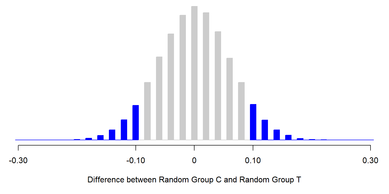
The p-value from the simulation will often not be exactly the same as the p-value from a statistical test. In some cases, this difference is because the random element of the simulation produces only an approximation of the p-value. In other cases, this difference is because the statistical test produces an approximation that is based on assumptions about the data that are not completely true.
For an example, let’s discuss another command that can be used to compare one sample proportion to another sample proportion: a two-sample proportion test. If we enter the statistics on our own, a form of a two-sample proportion test in Stata is…
prtesti N1 C1 N2 C2, count
…in which N1 is the sample size of Group 1, C1 is the number of successes in Group 1, N2 is the sample size of Group 2, and C2 is the number of successes in Group 2.
prtesti 100 70 100 80, count
running D:\OneDrive - IL State University\2-teaching\R for teaching\POL497\prof

> ile.do ...


Two-sample test of proportions                     x: Number of obs =      100
                                                   y: Number of obs =      100
------------------------------------------------------------------------------
             |       Mean   Std. Err.      z    P>|z|     [95% Conf. Interval]
-------------+----------------------------------------------------------------
           x |         .7   .0458258                      .6101832    .7898168
           y |         .8        .04                      .7216014    .8783986
-------------+----------------------------------------------------------------
        diff |        -.1   .0608276                       -.21922      .01922
             |  under Ho:   .0612372    -1.63   0.102
------------------------------------------------------------------------------
        diff = prop(x) - prop(y)                                  z =  -1.6330
    Ho: diff = 0

    Ha: diff < 0                 Ha: diff != 0                 Ha: diff > 0
 Pr(Z < z) = 0.0512         Pr(|Z| > |z|) = 0.1025          Pr(Z > z) = 0.9488
So instead of a two-tailed p-value of p=0.141 from the Fisher’s exact test, the two-tailed p-value is p=0.1025 from the two-sample proportion test. This two-sample proportion test produces an approximation that makes it relatively easy to calculate an estimated p-value, but isn’t needed if we have statistical software that can perform a Fisher’s exact test. The two-tailed p-values from a two-sample proportion test should approach the two-tailed p-value from Fisher’s exact test as sample sizes increase. For example:
tabi 30000 29950 \ 30000 30050, exact
running D:\OneDrive - IL State University\2-teaching\R for teaching\POL497\prof

> ile.do ...

           |          col
       row |         1          2 |     Total
-----------+----------------------+----------
         1 |    30,000     29,950 |    59,950
         2 |    30,000     30,050 |    60,050
-----------+----------------------+----------
     Total |    60,000     60,000 |   120,000

           Fisher's exact =                 0.777
   1-sided Fisher's exact =                 0.389
prtesti 60000 30000 60000 30050, count
running D:\OneDrive - IL State University\2-teaching\R for teaching\POL497\prof
> ile.do ...
Two-sample test of proportions x: Number of obs = 60000
y: Number of obs = 60000
------------------------------------------------------------------------------
| Mean Std. Err. z P>|z| [95% Conf. Interval]
-------------+----------------------------------------------------------------
x | .5 .0020412 .4959992 .5040008
y | .5008333 .0020412 .4968326 .5048341
-------------+----------------------------------------------------------------
diff | -.0008333 .0028867 -.0064913 .0048246
| under Ho: .0028868 -0.29 0.773
------------------------------------------------------------------------------
diff = prop(x) - prop(y) z = -0.2887
Ho: diff = 0
Ha: diff < 0 Ha: diff != 0 Ha: diff > 0
Pr(Z < z) = 0.3864 Pr(|Z| > |z|) = 0.7728 Pr(Z > z) = 0.6136Comparing a sample mean to a specific mean
The binomial test can be used to compared an observed proportion to a specific proportion. Proportions have two categories, such as whether a participant voted for Joe Biden or did not vote for Joe Biden. But outcomes can have more than two categories, such as participant ratings about Joe Biden on a scale from 0 for very cold to 100 for very warm, in which a participant can select 0 or 100 or any whole number between 0 and 100. For such outcomes, a t-test can be used to estimate a p-value. The one sample t-test can be used to test the null hypothesis that the mean in one sample equals a specific value. If we enter the statistics on our own, the form of a one-sample t-test in Stata is…
ttesti N MEAN SD VALUE
…in which N is the sample size, MEAN is the mean, SD is the standard deviation, and VALUE is the numeric value that we are testing for a difference from.
Let’s conduct a one-sample t-test. Let’s imagine that we ask a random sample of 90 U.S. residents to rate Joe Biden on a scale from 0 to 100, and the responses have a mean of 56 and standard deviation of 20. Let’s test the null hypothesis that the mean rating about Joe Biden in the population differs from 50.
ttesti 90 54 20 50
running D:\OneDrive - IL State University\2-teaching\R for teaching\POL497\prof

> ile.do ...


One-sample t test
------------------------------------------------------------------------------
         |     Obs        Mean    Std. Err.   Std. Dev.   [95% Conf. Interval]
---------+--------------------------------------------------------------------
       x |      90          54    2.108185          20    49.81108    58.18892
------------------------------------------------------------------------------
    mean = mean(x)                                                t =   1.8974
Ho: mean = 50                                    degrees of freedom =       89

    Ha: mean < 50               Ha: mean != 50                 Ha: mean > 50
 Pr(T < t) = 0.9695         Pr(|T| > |t|) = 0.0610          Pr(T > t) = 0.0305
Among these nine respondents, the mean rating about Joe Biden was 64, and the two-tailed p-value is 0.0610 for a test of the null hypothesis that, in the population, the mean rating of Joe Biden is 50. That’s not sufficient evidence at the conventional level in political science to conclude that the population mean differs from 50. But the p-value is close to p=0.05, so we can interpret that as somewhat strong evidence against the null hypothesis.
Comparing a sample mean to another sample mean
The two sample t-test can be used to test the null hypothesis that the mean in one population equals the mean in another population. But, in some situations, this comparison can be handled in two ways: in a unpaired comparison, the observations in one group are treated as independent of the observations in the other group; but in a paired comparison, the observations in one group are matched with the observations in the other group.
Let’s use data from a hypothetical class, in which eleven students at the start of the semester took a 12-item multiple-choice pretest, and then, at the end of the semester, the same eleven students took the same 12-item multiple-choice test as a posttest. The unpaired t-test will compare the mean pretest score to the mean posttest score, without regard for matching pretest scores to posttest scores for each student:
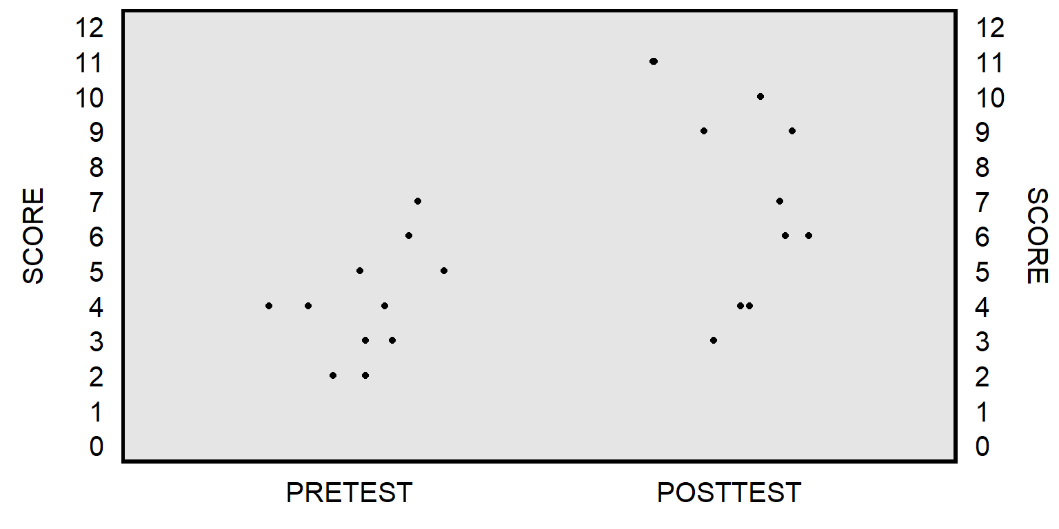
The paired t-test will instead match the pretest score for each student to the posttest score for that student to get a pretest-to-posttest change in score for each student, and then test whether the mean pretest-to-posttest change in scores equals zero:
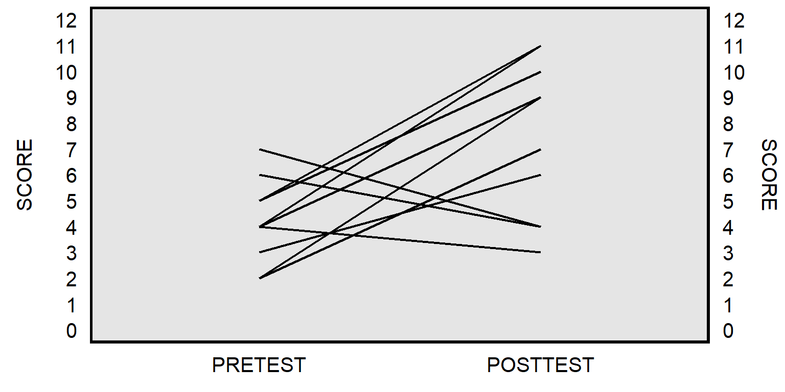
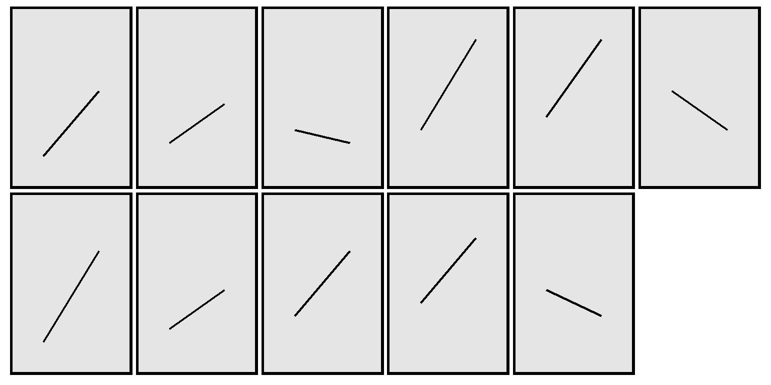
The plot above isn’t ideal because the line for one student might be on top of the line for another student, if multiple students had the same pretest score and posttest score. Below is a better representation, by student:
If we enter the statistics on our own, the form of a two-sample unpaired t-test in Stata is…
ttesti N1 MEAN1 SD1 N2 MEAN2 SD2
…in which N is the sample size, MEAN is the mean, SD is the standard deviation, with the 1 and 2 indicating the sample. Let’s add an “unequal” option, which tells Stata to not assume that the standard deviation of the groups equal each other.
ttesti 11 4.091 1.578 11 7.273 2.901, unequal
running D:\OneDrive - IL State University\2-teaching\R for teaching\POL497\prof

> ile.do ...


Two-sample t test with unequal variances
------------------------------------------------------------------------------
         |     Obs        Mean    Std. Err.   Std. Dev.   [95% Conf. Interval]
---------+--------------------------------------------------------------------
       x |      11       4.091    .4757849       1.578    3.030885    5.151115
       y |      11       7.273    .8746844       2.901    5.324082    9.221918
---------+--------------------------------------------------------------------
combined |      22       5.682     .597156     2.80091    4.440146    6.923854
---------+--------------------------------------------------------------------
    diff |              -3.182    .9957129               -5.299041   -1.064959
------------------------------------------------------------------------------
    diff = mean(x) - mean(y)                                      t =  -3.1957
Ho: diff = 0                     Satterthwaite's degrees of freedom =  15.4413

    Ha: diff < 0                 Ha: diff != 0                 Ha: diff > 0
 Pr(T < t) = 0.0029         Pr(|T| > |t|) = 0.0058          Pr(T > t) = 0.9971
The “i” at the end of the Stata commands bitesti, tabi, prtesti, and ttesti indicates that the command is an “immediate” command in which data for the test are entered in the command instead of drawn from memory in Stata. Let’s run an unpaired t-test command that uses data that has been loaded into Stata’s memory:
clear all
use ".\files\prepost.dta"
ttest POSTTEST = PRETEST, unpaired unequal
running D:\OneDrive - IL State University\2-teaching\R for teaching\POL497\prof

> ile.do ...


Two-sample t test with unequal variances
------------------------------------------------------------------------------
Variable |     Obs        Mean    Std. Err.   Std. Dev.   [95% Conf. Interval]
---------+--------------------------------------------------------------------
POSTTEST |      11    7.272727    .8748081     2.90141    5.323533    9.221921
 PRETEST |      11    4.090909    .4758637    1.578261    3.030619      5.1512
---------+--------------------------------------------------------------------
combined |      22    5.681818    .5972026    2.801128    4.439867    6.923769
---------+--------------------------------------------------------------------
    diff |            3.181818    .9958592                1.064468    5.299168
------------------------------------------------------------------------------
    diff = mean(POSTTEST) - mean(PRETEST)                         t =   3.1950
Ho: diff = 0                     Satterthwaite's degrees of freedom =  15.4415

    Ha: diff < 0                 Ha: diff != 0                 Ha: diff > 0
 Pr(T < t) = 0.9971         Pr(|T| > |t|) = 0.0058          Pr(T > t) = 0.0029
For a paired t-test in Stata, the “unequal” option isn’t needed:
ttest POSTTEST = PRETEST
running D:\OneDrive - IL State University\2-teaching\R for teaching\POL497\prof

> ile.do ...


Paired t test
------------------------------------------------------------------------------
Variable |     Obs        Mean    Std. Err.   Std. Dev.   [95% Conf. Interval]
---------+--------------------------------------------------------------------
POSTTEST |      11    7.272727    .8748081     2.90141    5.323533    9.221921
 PRETEST |      11    4.090909    .4758637    1.578261    3.030619      5.1512
---------+--------------------------------------------------------------------
    diff |      11    3.181818    1.085593    3.600505     .762966     5.60067
------------------------------------------------------------------------------
     mean(diff) = mean(POSTTEST - PRETEST)                        t =   2.9309
 Ho: mean(diff) = 0                              degrees of freedom =       10

 Ha: mean(diff) < 0           Ha: mean(diff) != 0           Ha: mean(diff) > 0
 Pr(T < t) = 0.9925         Pr(|T| > |t|) = 0.0150          Pr(T > t) = 0.0075
The p-value for the unpaired t-test (p=0.0058) is lower than the p-value for the paired t-test (p=0.0150), indicating that the unpaired analysis provided more evidence against the corresponding null hypotheses than the paired analysis provided. But the p-value for an unpaired t-test will not always be lower than the p-value for a paired t-test: it depends on whether the pairing of the observations produces more or less evidence against the null hypothesis.
For the analysis below, I kept the pretest scores and posttest scores the same, but I shuffled the pairings, so that the pretest-to-posttest change more consistently indicated improvement from pretest to posttest:
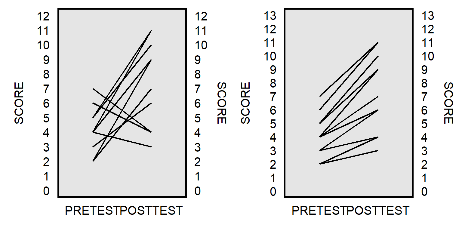
clear all
use ".\files\prepost SHUFFLED.dta"
ttest POSTTEST = PRETEST
running D:\OneDrive - IL State University\2-teaching\R for teaching\POL497\prof

> ile.do ...


Paired t test
------------------------------------------------------------------------------
Variable |     Obs        Mean    Std. Err.   Std. Dev.   [95% Conf. Interval]
---------+--------------------------------------------------------------------
POSTTEST |      11    7.272727    .8748081     2.90141    5.323533    9.221921
 PRETEST |      11    4.090909    .4758637    1.578261    3.030619      5.1512
---------+--------------------------------------------------------------------
    diff |      11    3.181818    .4635472    1.537412    2.148971    4.214666
------------------------------------------------------------------------------
     mean(diff) = mean(POSTTEST - PRETEST)                        t =   6.8641
 Ho: mean(diff) = 0                              degrees of freedom =       10

 Ha: mean(diff) < 0           Ha: mean(diff) != 0           Ha: mean(diff) > 0
 Pr(T < t) = 1.0000         Pr(|T| > |t|) = 0.0000          Pr(T > t) = 0.0000
The p-value for the unpaired t-test is still p=0.0058, but the p-value for the shuffled paired t-test is smaller, rounding to p=0.0000 to four decimal places.
Sample practice items
Among the 30 students in a POL 138 section who took the multiple-choice pretest at the start of the semester and then took the same multiple-choice test as a posttest at the end of the semester, the mean pretest score was 4.0, the mean posttest score was 8.4, and the p-value was p<0.05 for an unpaired t-test of the null hypothesis that the mean pretest score equals the mean posttest score. Is this sufficient evidence at the conventional level in political science to conclude that, at least on average, these students learned something about the POL 138 content on the test?
- Yes
- No
Answer
- Yes
There are two possible explanations for the difference between the 4.0 pretest mean score and the 8.4 posttest mean score: [1] the students on average learned more about the POL 138 content, and [2] the students by random luck happened to guess more correct responses on the posttest than on the pretest. But the p-value under p=0.05 permits us to eliminate random guessing as a plausible explanation at the conventional level in political science, so the only other plausible explanation is that the students on average learned more about the POL 138 content.
Review of selected tests
| Test | Use |
|---|---|
| Binomial test | Comparing a sample proportion to a specific proportion |
| Fisher’s exact test | Comparing one sample proportion to another sample proportion |
| One-sample t-test | Comparing a sample mean to a specific mean |
| Two-sample t-test | Comparing a sample mean to another sample mean |
16.7 Stata programming
For running the commands below, import to Stata the Shay_and_Rauhaus_LSQ.csv file at the Dataverse page for Shay and Rauhaus 2023.
Loops
levelsof fip, local(STATES)
foreach i of local STATES {
  display `"--- State `i'"'
  ci mean pctwomenearn pctwomenleg if fip==`i'
 }
Write to another file
tempname STATEFILE
   postfile `STATEFILE' fip coeff se using "D:REGSTATE.dta", replace
   levelsof fip, local(STATES)
   foreach i of local STATES {
     reg pctwomenearn pctwomenleg if fip==`i', robust
     post `STATEFILE' (`i') (_b[pctwomenleg]) (_se[pctwomenleg])
   }
postclose `STATEFILE'
Write to another file and calculate 95% confidence intervals
gen cilo = .
gen cihi = .
tempname STATEFILE
   postfile `STATEFILE' fip coeff se cilo cihi using "D:REGSTATE.dta", replace
   levelsof fip, local(STATES)
   foreach i of local STATES {
     reg pctwomenearn pctwomenleg if fip==`i', robust
     replace cilo = _b[pctwomenleg] - invttail(`e(df_r)',0.025)*_se[pctwomenleg]
     replace cihi = _b[pctwomenleg] + invttail(`e(df_r)',0.025)*_se[pctwomenleg]
     post `STATEFILE' (`i') (_b[pctwomenleg]) (_se[pctwomenleg]) (cilo) (cihi)
   }
postclose `STATEFILE'

* Check
help reg
reg pctwomenearn pctwomenleg if fip==25, robust
16.8 Panel analysis
Panel data have multiple observations from a case over time, such as survey participants completing a survey each year for three years or observations of a set of countries each year over a decade. These observations are not independent, and the analysis should account for this.
For an illustration, the plot below has 12 points and a line of best fit through the points. The predictor is X and the outcome is Y.
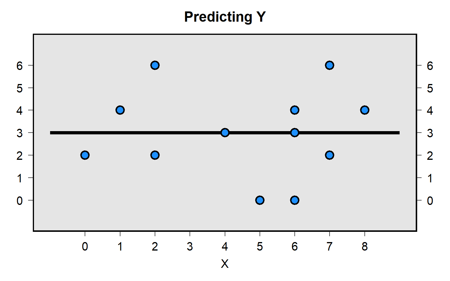
The regression output below is for the plot above, indicating that the slope of the line is flat (0.00):
reg Y X
running D:\OneDrive - IL State University\2-teaching\R for teaching\POL497\prof

> ile.do ...

      Source |       SS           df       MS      Number of obs   =        12
-------------+----------------------------------   F(1, 10)        =      0.00
       Model |           0         1           0   Prob > F        =    1.0000
    Residual |          42        10         4.2   R-squared       =    0.0000
-------------+----------------------------------   Adj R-squared   =   -0.1000
       Total |          42        11  3.81818182   Root MSE        =    2.0494

------------------------------------------------------------------------------
           Y |      Coef.   Std. Err.      t    P>|t|     [95% Conf. Interval]
-------------+----------------------------------------------------------------
           X |      0.000      0.234     0.00   1.000       -0.520       0.520
       _cons |      3.000      1.206     2.49   0.032        0.313       5.687
------------------------------------------------------------------------------
But suppose that the 12 points were not independent of each other but were rather drawn only from four countries – A, B, C, and D – with each country having a point from the year 2010, another point from the year 2011, and another point from the year 2012. The plot below indicates that, even though the overall association between X and Y is zero across all 12 points, the patterns within country indicate that higher X associates with higher Y:
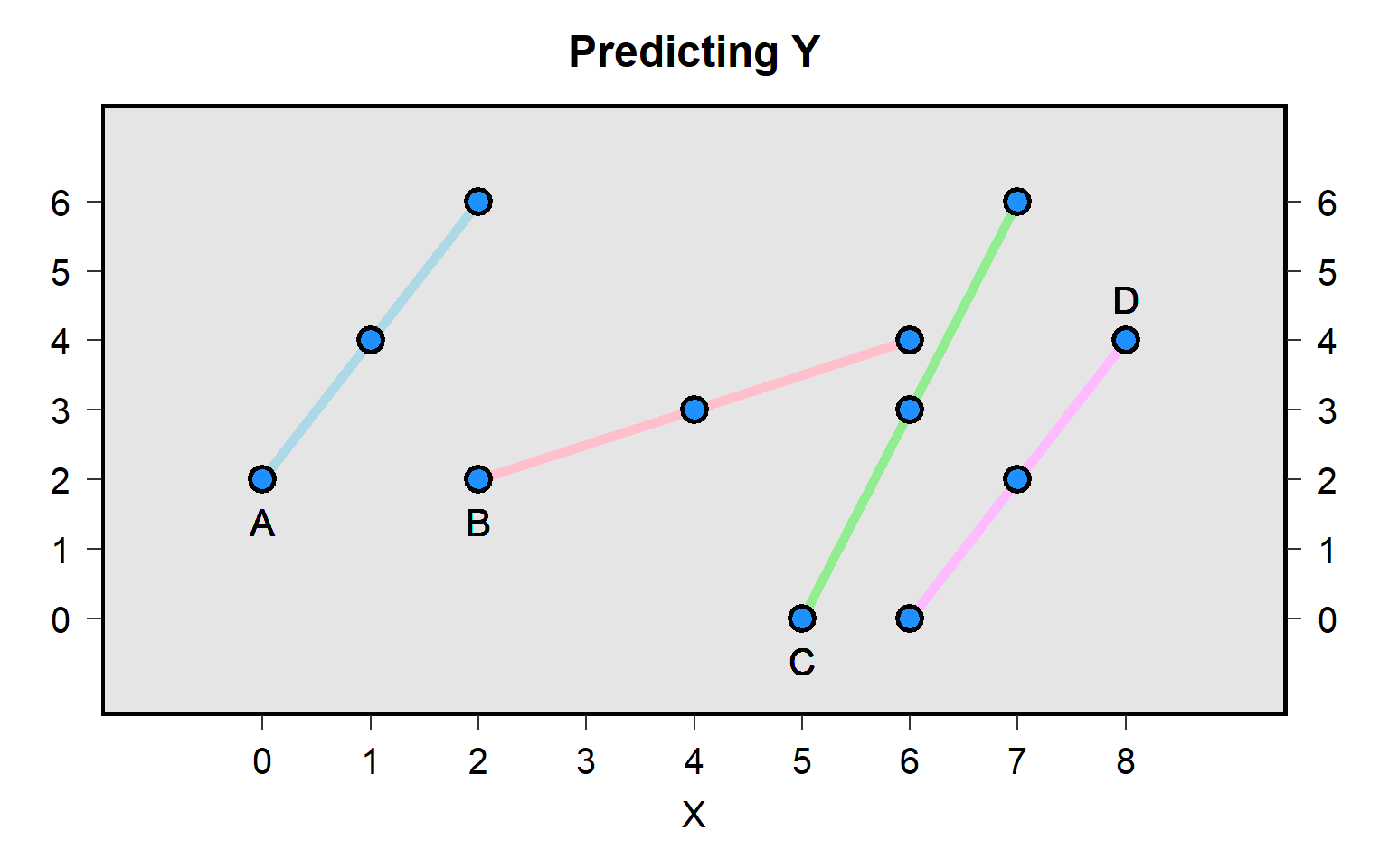
The output below is limited to the association between X and Y within countries:
xtset COUNTRYCODE YEAR

xtreg Y X, fe
running D:\OneDrive - IL State University\2-teaching\R for teaching\POL497\prof

> ile.do ...

       panel variable:  COUNTRYCODE (strongly balanced)
        time variable:  YEAR, 2010 to 2012
                delta:  1 unit


Fixed-effects (within) regression               Number of obs     =         12
Group variable: COUNTRYCODE                     Number of groups  =          4

R-sq:                                           Obs per group:
     within  = 0.6429                                         min =          3
     between = 0.8571                                         avg =        3.0
     overall = 0.0000                                         max =          3

                                                F(1,7)            =      12.60
corr(u_i, Xb)  = -0.9021                        Prob > F          =     0.0093

------------------------------------------------------------------------------
           Y |      Coef.   Std. Err.      t    P>|t|     [95% Conf. Interval]
-------------+----------------------------------------------------------------
           X |      1.286      0.362     3.55   0.009        0.429       2.142
       _cons |     -2.786      1.676    -1.66   0.140       -6.749       1.178
-------------+----------------------------------------------------------------
     sigma_u |  4.1690469
     sigma_e |  1.3552619
         rho |  .90442478   (fraction of variance due to u_i)
------------------------------------------------------------------------------
F test that all u_i=0: F(3, 7) = 5.29                        Prob > F = 0.0322
For panel analysis, a fixed-effects regression uses information from the predictors that vary within country but does not use information from predictors that vary between countries. However, a random-effects regression uses information from the predictors that vary within country and from predictors that vary between countries.
For a random-effects regression predictor in which the value of the predictor changes within country and between countries, the coefficient indicates the predicted change in the outcome variable when the predictor increases one unit within and between countries, holding other model predictors constant. For a random effects regression predictor in which the value of the predictor does not change within country, the coefficient indicates the predicted change in the outcome variable when the predictor increases one unit between countries, holding other model predictors constant.
xtreg Y X, re
running D:\OneDrive - IL State University\2-teaching\R for teaching\POL497\prof

> ile.do ...


Random-effects GLS regression                   Number of obs     =         12
Group variable: COUNTRYCODE                     Number of groups  =          4

R-sq:                                           Obs per group:
     within  = 0.0000                                         min =          3
     between = 0.0000                                         avg =        3.0
     overall = 0.0000                                         max =          3

                                                Wald chi2(1)      =       0.00
corr(u_i, X)   = 0 (assumed)                    Prob > chi2       =     1.0000

------------------------------------------------------------------------------
           Y |      Coef.   Std. Err.      z    P>|z|     [95% Conf. Interval]
-------------+----------------------------------------------------------------
           X |      0.000      0.234     0.00   1.000       -0.458       0.458
       _cons |      3.000      1.206     2.49   0.013        0.636       5.364
-------------+----------------------------------------------------------------
     sigma_u |          0
     sigma_e |  1.3552619
         rho |          0   (fraction of variance due to u_i)
------------------------------------------------------------------------------
16.9 Dataset shapes for repeated observations
For datasets that contain multiple observations per each person, country, or other thing, there are two basic ways to set up the dataset. Let’s use a simple example of two students (A and B), who each take the same test at three points in time (t1, T2, and t3).
The long shape for the data would look something like this:
STUDENT  TIME   SCORE
   A      T1      70
   A      T2      75
   A      T3      76
   B      T1      80
   B      T2      79
   B      T3      81
The wide shape for the data would look something like this:
STUDENT  SCORE1 SCORE2 SCORE3
   A       70     75     76
   B       80     79     81
The reshape command in Stata can be used to convert from wide to long or from long to wide.
16.10 Panel analysis in Stata
Let’s import the data for Shay and Rauhaus 2023 “Closing the Gap: An Analysis of Women’s Representation in State Legislatures and the Gender Pay Gap”:
clear all

import delimited "./files/Shay_and_Rauhaus_LSQ.csv", case(upper)
running D:\OneDrive - IL State University\2-teaching\R for teaching\POL497\prof

> ile.do ...


(19 vars, 650 obs)
Let’s set up the panel setup for Stata:
xtset FIP YEAR
running D:\OneDrive - IL State University\2-teaching\R for teaching\POL497\prof

> ile.do ...

       panel variable:  FIP (strongly balanced)
        time variable:  YEAR, 2004 to 2016
                delta:  1 unit
Let’s run a fixed effects regression:
xtreg PCTWOMENEARN PCTWOMENLEG CITIZEN_IDEOL GOVT_IDEOL UNEMPLOYMENT POVERTY_RATE GSP INCOME EVANGLE IG_WOMEN_PCT STATEMIN LEG_PROF i.YEAR, fe
running D:\OneDrive - IL State University\2-teaching\R for teaching\POL497\prof

> ile.do ...


note: EVANGLE omitted because of collinearity
note: LEG_PROF omitted because of collinearity

Fixed-effects (within) regression               Number of obs     =        400
Group variable: FIP                             Number of groups  =         50

R-sq:                                           Obs per group:
     within  = 0.1402                                         min =          8
     between = 0.0583                                         avg =        8.0
     overall = 0.0249                                         max =          8

                                                F(16,334)         =       3.40
corr(u_i, Xb)  = -0.7568                        Prob > F          =     0.0000

------------------------------------------------------------------------------
PCTWOMENEARN |      Coef.   Std. Err.      t    P>|t|     [95% Conf. Interval]
-------------+----------------------------------------------------------------
 PCTWOMENLEG |      0.150      0.067     2.25   0.025        0.019       0.281
CITIZEN_ID~L |     -0.058      0.033    -1.75   0.081       -0.124       0.007
  GOVT_IDEOL |     -0.022      0.019    -1.16   0.248       -0.059       0.015
UNEMPLOYMENT |     -0.474      0.207    -2.29   0.022       -0.881      -0.068
POVERTY_RATE |      0.006      0.125     0.05   0.960       -0.240       0.252
         GSP |     -3.626      3.138    -1.16   0.249       -9.799       2.547
      INCOME |     -0.000      0.000    -0.84   0.402       -0.000       0.000
     EVANGLE |      0.000  (omitted)
IG_WOMEN_PCT |     46.413     36.377     1.28   0.203      -25.144     117.971
    STATEMIN |      0.249      0.330     0.75   0.451       -0.400       0.899
    LEG_PROF |      0.000  (omitted)
             |
        YEAR |
       2005  |      1.376      0.570     2.41   0.016        0.255       2.497
       2006  |      1.064      0.782     1.36   0.175       -0.475       2.603
       2007  |      1.812      1.064     1.70   0.090       -0.282       3.906
       2008  |      2.272      1.396     1.63   0.105       -0.474       5.018
       2009  |      2.691      1.378     1.95   0.052       -0.019       5.402
       2010  |      4.115      1.817     2.26   0.024        0.540       7.689
       2011  |      5.175      2.214     2.34   0.020        0.819       9.531
             |
       _cons |    125.853     38.561     3.26   0.001       49.999     201.707
-------------+----------------------------------------------------------------
     sigma_u |  6.3210878
     sigma_e |  2.4694738
         rho |  .86758499   (fraction of variance due to u_i)
------------------------------------------------------------------------------
F test that all u_i=0: F(49, 334) = 16.03                    Prob > F = 0.0000
Let’s run a random effects regression:
xtreg PCTWOMENEARN PCTWOMENLEG CITIZEN_IDEOL GOVT_IDEOL UNEMPLOYMENT POVERTY_RATE GSP INCOME EVANGLE IG_WOMEN_PCT STATEMIN LEG_PROF i.YEAR, re
running D:\OneDrive - IL State University\2-teaching\R for teaching\POL497\prof

> ile.do ...


Random-effects GLS regression                   Number of obs     =        400
Group variable: FIP                             Number of groups  =         50

R-sq:                                           Obs per group:
     within  = 0.1307                                         min =          8
     between = 0.1907                                         avg =        8.0
     overall = 0.1744                                         max =          8

                                                Wald chi2(18)     =      61.17
corr(u_i, X)   = 0 (assumed)                    Prob > chi2       =     0.0000

------------------------------------------------------------------------------
PCTWOMENEARN |      Coef.   Std. Err.      z    P>|z|     [95% Conf. Interval]
-------------+----------------------------------------------------------------
 PCTWOMENLEG |      0.162      0.054     2.97   0.003        0.055       0.268
CITIZEN_ID~L |     -0.016      0.029    -0.55   0.581       -0.073       0.041
  GOVT_IDEOL |     -0.022      0.018    -1.26   0.207       -0.057       0.012
UNEMPLOYMENT |     -0.441      0.185    -2.38   0.017       -0.804      -0.079
POVERTY_RATE |      0.075      0.111     0.67   0.502       -0.144       0.293
         GSP |      0.693      0.529     1.31   0.190       -0.343       1.730
      INCOME |     -0.000      0.000    -1.01   0.313       -0.000       0.000
     EVANGLE |     -0.052      0.064    -0.81   0.420       -0.177       0.074
IG_WOMEN_PCT |     47.174     35.220     1.34   0.180      -21.856     116.204
    STATEMIN |      0.449      0.299     1.50   0.134       -0.138       1.035
    LEG_PROF |      5.091      5.330     0.96   0.339       -5.355      15.537
             |
        YEAR |
       2005  |      0.989      0.524     1.89   0.059       -0.038       2.017
       2006  |      0.377      0.617     0.61   0.541       -0.832       1.586
       2007  |      0.603      0.765     0.79   0.430       -0.895       2.102
       2008  |      0.623      0.954     0.65   0.514       -1.246       2.492
       2009  |      1.068      0.872     1.22   0.221       -0.642       2.778
       2010  |      2.622      1.289     2.03   0.042        0.095       5.149
       2011  |      3.386      1.567     2.16   0.031        0.315       6.457
             |
       _cons |     70.671      8.934     7.91   0.000       53.161      88.181
-------------+----------------------------------------------------------------
     sigma_u |  3.6162718
     sigma_e |  2.4694738
         rho |  .68197804   (fraction of variance due to u_i)
------------------------------------------------------------------------------
Let’s use a local to avoid long sets of controls in our regression command:
local CONTROLS PCTWOMENLEG CITIZEN_IDEOL GOVT_IDEOL UNEMPLOYMENT POVERTY_RATE GSP INCOME EVANGLE IG_WOMEN_PCT STATEMIN LEG_PROF i.YEAR

xtreg PCTWOMENEARN `CONTROLS', re
running D:\OneDrive - IL State University\2-teaching\R for teaching\POL497\prof

> ile.do ...


Random-effects GLS regression                   Number of obs     =        400
Group variable: FIP                             Number of groups  =         50

R-sq:                                           Obs per group:
     within  = 0.1307                                         min =          8
     between = 0.1907                                         avg =        8.0
     overall = 0.1744                                         max =          8

                                                Wald chi2(18)     =      61.17
corr(u_i, X)   = 0 (assumed)                    Prob > chi2       =     0.0000

------------------------------------------------------------------------------
PCTWOMENEARN |      Coef.   Std. Err.      z    P>|z|     [95% Conf. Interval]
-------------+----------------------------------------------------------------
 PCTWOMENLEG |      0.162      0.054     2.97   0.003        0.055       0.268
CITIZEN_ID~L |     -0.016      0.029    -0.55   0.581       -0.073       0.041
  GOVT_IDEOL |     -0.022      0.018    -1.26   0.207       -0.057       0.012
UNEMPLOYMENT |     -0.441      0.185    -2.38   0.017       -0.804      -0.079
POVERTY_RATE |      0.075      0.111     0.67   0.502       -0.144       0.293
         GSP |      0.693      0.529     1.31   0.190       -0.343       1.730
      INCOME |     -0.000      0.000    -1.01   0.313       -0.000       0.000
     EVANGLE |     -0.052      0.064    -0.81   0.420       -0.177       0.074
IG_WOMEN_PCT |     47.174     35.220     1.34   0.180      -21.856     116.204
    STATEMIN |      0.449      0.299     1.50   0.134       -0.138       1.035
    LEG_PROF |      5.091      5.330     0.96   0.339       -5.355      15.537
             |
        YEAR |
       2005  |      0.989      0.524     1.89   0.059       -0.038       2.017
       2006  |      0.377      0.617     0.61   0.541       -0.832       1.586
       2007  |      0.603      0.765     0.79   0.430       -0.895       2.102
       2008  |      0.623      0.954     0.65   0.514       -1.246       2.492
       2009  |      1.068      0.872     1.22   0.221       -0.642       2.778
       2010  |      2.622      1.289     2.03   0.042        0.095       5.149
       2011  |      3.386      1.567     2.16   0.031        0.315       6.457
             |
       _cons |     70.671      8.934     7.91   0.000       53.161      88.181
-------------+----------------------------------------------------------------
     sigma_u |  3.6162718
     sigma_e |  2.4694738
         rho |  .68197804   (fraction of variance due to u_i)
------------------------------------------------------------------------------
Below is a different random effects estimation technique. Code from Shay and Rauhaus 2023, with me adding “noatlegend”:
xtpcse PCTWOMENEARN `CONTROLS', correlation(ar1)
running D:\OneDrive - IL State University\2-teaching\R for teaching\POL497\prof

> ile.do ...


(note: estimates of rho outside [-1,1] bounded to be in the range [-1,1])

Prais-Winsten regression, correlated panels corrected standard errors (PCSEs)

Group variable:   FIP                           Number of obs     =        400
Time variable:    YEAR                          Number of groups  =         50
Panels:           correlated (balanced)         Obs per group:
Autocorrelation:  common AR(1)                                min =          8
                                                              avg =          8
                                                              max =          8
Estimated covariances      =      1275          R-squared         =     0.8974
Estimated autocorrelations =         1          Wald chi2(0)      =          .
Estimated coefficients     =         1          Prob > chi2       =          .

------------------------------------------------------------------------------
             |           Panel-corrected
PCTWOMENEARN |      Coef.   Std. Err.      z    P>|z|     [95% Conf. Interval]
-------------+----------------------------------------------------------------
       _cons |     79.094      0.439   180.31   0.000       78.234      79.954
-------------+----------------------------------------------------------------
         rho |   .5616973
------------------------------------------------------------------------------
margins, at (PCTWOMENLEG=(8 (2) 42)) atmeans noatlegend
running D:\OneDrive - IL State University\2-teaching\R for teaching\POL497\prof
> ile.do ...
Adjusted predictions Number of obs = 400
Model VCE : Panel-corrected
Expression : Fitted values, predict()
------------------------------------------------------------------------------
| Delta-method
| Margin Std. Err. z P>|z| [95% Conf. Interval]
-------------+----------------------------------------------------------------
_at |
1 | 76.374 0.672 113.67 0.000 75.057 77.691
2 | 76.729 0.583 131.56 0.000 75.586 77.872
3 | 77.084 0.495 155.87 0.000 76.114 78.053
4 | 77.438 0.406 190.79 0.000 76.643 78.234
5 | 77.793 0.317 245.25 0.000 77.171 78.415
6 | 78.147 0.229 341.97 0.000 77.700 78.595
7 | 78.502 0.140 561.33 0.000 78.228 78.776
8 | 78.857 0.051 1540.90 0.000 78.756 78.957
9 | 79.211 0.037 2112.41 0.000 79.138 79.285
10 | 79.566 0.126 630.62 0.000 79.319 79.813
11 | 79.921 0.215 371.99 0.000 79.500 80.342
12 | 80.275 0.304 264.48 0.000 79.680 80.870
13 | 80.630 0.392 205.59 0.000 79.861 81.399
14 | 80.984 0.481 168.41 0.000 80.042 81.927
15 | 81.339 0.570 142.82 0.000 80.223 82.455
16 | 81.694 0.658 124.11 0.000 80.404 82.984
17 | 82.048 0.747 109.85 0.000 80.584 83.512
18 | 82.403 0.836 98.62 0.000 80.765 84.041
------------------------------------------------------------------------------marginsplot, recast(line) recastci(rarea)
running D:\OneDrive - IL State University\2-teaching\R for teaching\POL497\prof
> ile.do ...
Variables that uniquely identify margins: PCTWOMENLEG