11 Threats to Inference 2
11.1 Misinterpreting p>0.05
Major learning objective(s) for this section:
- Know that the lack of statistical significance does not necessarily mean the lack of an effect.
- Know how to use 95% confidence intervals to assess the informational value of null results.
Remember that a p-value is a measure of the strength of evidence that an analysis has provided against a null hypothesis. For political science, a p-value under p=0.05 is sufficient to reject the null hypothesis. A common error of inference is to interpret a p-value that is not under p=0.05 as evidence that the null hypothesis is true. For instance, suppose that we flipped a coin 3 times and got 3 heads and 0 tails. The p-value would be p=0.25 for a test of the null hypothesis that the coin is fair, so that there is not enough evidence to reject the null hypothesis that the coin is fair. But that doesn’t mean that there is enough evidence to infer that the coin is fair: after all, the coin never landed on tails!
For a published example of this, Ono and Zilis 2021 reported on a list experiment that attempted to measure percentages of respondents that agreed with the statement that “When a court case concerns issues like immigration, some Hispanic judges might give biased rulings”. For a test of the null hypothesis that zero percent of Hispanics agreed with that statement, the p-value was not under p=0.05. Ono and Zilis 2021 suggested (p. 4) that:
Hispanics do not believe that Hispanic judges are biased.
However, the estimate from the analysis was that 25% of Hispanics agreed with the statement, so the p-value not being under p=0.05 does not mean that the relatively large 25% estimate should be treated as if it were zero. The figure below presents the 95% confidence interval for this 25% estimate, which suggests that – while the analysis did not provide sufficient evidence that the percentage agreement among Hispanics differs from zero – the analysis also did not provide sufficient evidence that the percentage agreement was zero or was even close to zero. The 95% confidence interval indicates that 0% cannot be excluded as a plausible value, but 50% cannot be excluded as a plausible value, either.
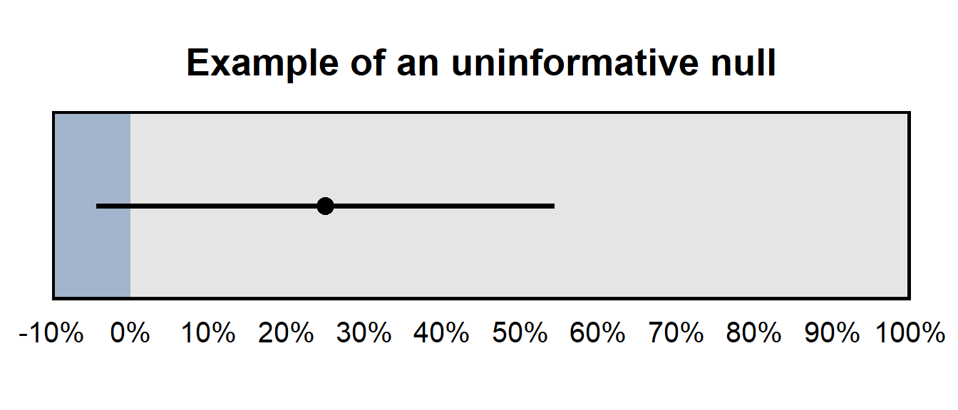
The 95% confidence interval was [-4%, 54%] for the percentage of Hispanics who agreed with the statement, so the analysis did not provide a precise estimate of the percentage of Hispanics who agreed with the statement. This type of imprecise estimate that contains zero can be referred to as an an uninformative null, which means that the analysis did not provide sufficient evidence to reject zero as a plausible value (which makes that a “null” result), and the analysis did not provide sufficient evidence to rule out large estimates as implausible, so the analysis did not provide much information about the what the true number is (which makes the analysis uninformative).
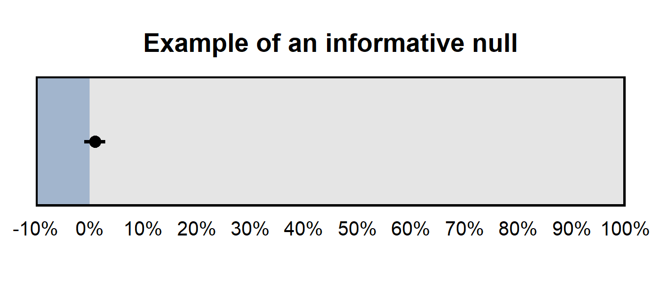
But if the 95% confidence interval has been, say, [-1%, 3%], that would have been an informative null, because – even though the analysis did not provide sufficient evidence to reject zero as a plausible value – the analysis did provide sufficient evidence to rule out large estimates as implausible.
Sample practice items
Of the things in the list below, which would be most useful for assessing whether a null result is an informative null?
- a p-value
- a point estimate
- a 95% confidence interval
Answer
- a 95% confidence interval
Suppose that our outcome is measured on a scale from 0 to 10. Which of the following 95% confidence intervals would be a more informative null, for a treatment effect?
- [-1,2]
- [-40,40]
Answer
- [-1,2]
[-1,2] is a more informative null than [-40,40] is because the ends of [-1,2] is closer to zero.
11.2 Misinterpreting differences in statistical significance
A common bad inference is to infer a difference between estimates merely because the p-value for one estimate falls below a p-value threshold (and is thus “statistically significant”) and the p-value for the other p-value does not fall below that threshold (and is thus not “statistically significant”). This is a bad inference because, to infer something about the difference between estimates, we should have a p-value about that difference in estimates. p-values about each inference aren’t useful for making an inference about the difference between the estimates.
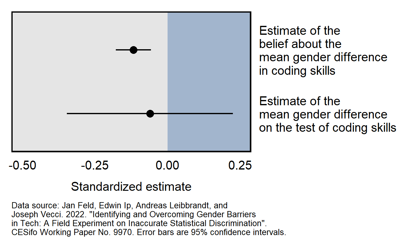
Consider the Feld et al 2022 working paper, which reported that:
We find evidence consistent with inaccurate statistical discrimination: while there are no significant gender differences in performance, employers believe that female programmers perform worse than male programmers.
Results from the working paper are plotted below. The top 95% confidence interval does not cross zero and indicates that there is sufficient evidence to conclude that employers on average thought that the female programmers would perform worse than the male programmers would perform. The bottom 95% confidence interval crosses zero, which means that the analysis did not provide sufficient evidence to conclude that female programmers performed worse than male programmers performed. However, the estimate of the male/female difference in test performance is so imprecise that we can’t conclude with any reasonable confidence that the employers were incorrect in their perception that female programmers would perform worse than the male programmers.
Sample practice items
Suppose that researchers have a sample of men participants and women participants and test the effect of a treatment on the participants. Results provide evidence at p=0.03 that the treatment worked among men, but the p-value is p=0.20 for the test of the effect among women. Is this sufficient evidence to support the conclusion that the treatment was more effective among men than among women?
- Yes: the p-values of p=0.03 and p=0.20 provide sufficient evidence that the treatment worked among men but did not provide sufficient evidence that the treatment worked among women.
- No: p-values do not directly indicate anything about effect sizes, so we cannot conclude based on these p-values that the effect size was larger for men than for women.
Answer
- No: p-values do not directly indicate anything about effect sizes, so we cannot conclude based on these p-values that the effect size was larger for men than for women.
Suppose that, in a linear regression, the coefficient for a predictor of respondent education is 0.20, and the coefficient for a predictor of respondent age is 0.03. Both coefficients are statistically significant. Does this mean that that education has a larger predicted effect on the outcome than age has?
- Yes, because the coefficient for education is larger than the coefficient for age.
- No, because, even though the coefficient for education is larger than the coefficient for age, we need to know the scale of the predictors to assess how big an estimated effect each are.
Answer
B. No, because, even though the coefficient for education is larger than the coefficient for age, we need to know the scale of the predictors to assess how big an estimated effect each are.11.3 Multiple testing
Major learning objective(s) for this section:
- Discuss how inferences can be biased by multiple testing.
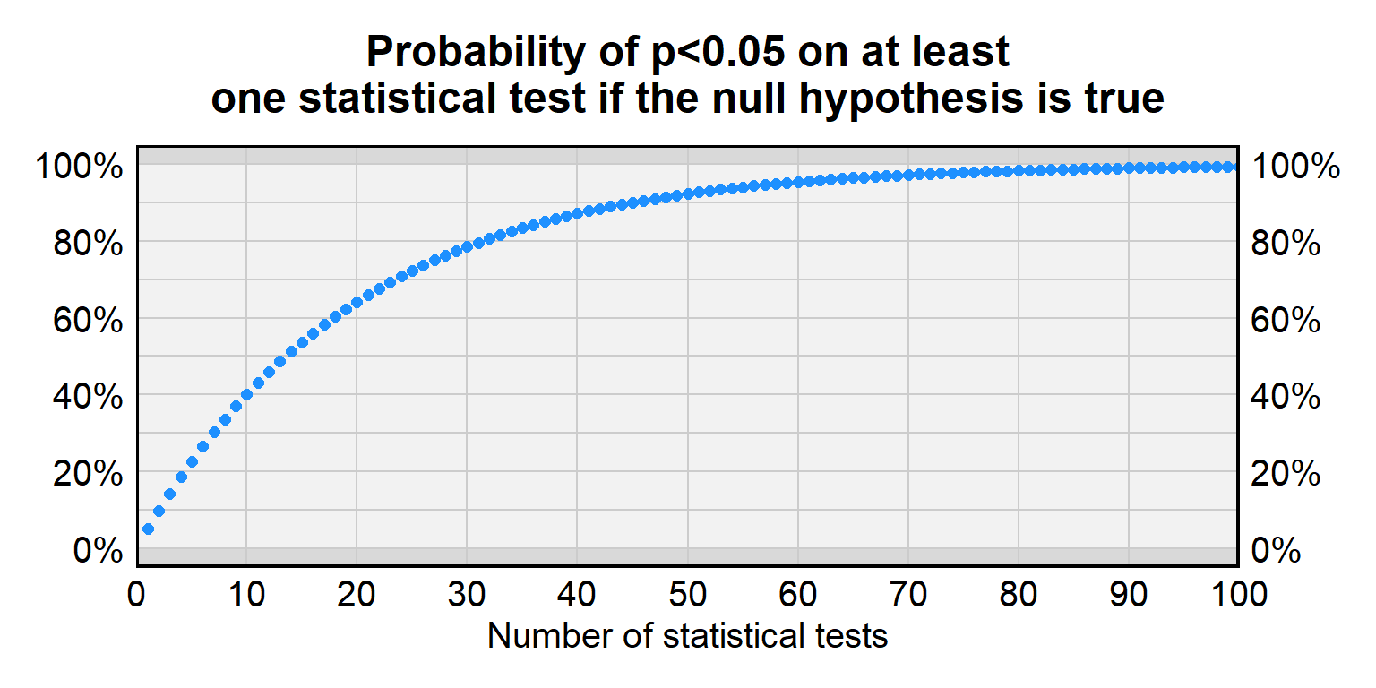
A p-value under p=0.05 sometimes occurs even if a treatment has no effect. In random data, the p-value will be p=0.05 or lower for 5% of statistical tests. But this 5% chance of incorrectly rejecting the null hypothesis is for a single statistical test, and, the more statistical tests we conduct for treatments that have no effect, the higher than chance that at least one of the p-values will be less than p=0.05. The problem of multiple testing is when researchers conduct a lot of statistical tests so that a small p-value for one of the tests becomes more likely to be due to random chance.
For a single test of a true null hypothesis, there is a 5% chance of incorrectly rejecting the null hypothesis and a 95% chance of correctly not rejecting the null hypothesis. For two tests of a true null hypothesis, the probability of correctly not rejecting the null hypothesis both times is \(0.95\times0.95\), which is only about 90%. For ten tests of a true null hypothesis, the probability of correctly not rejecting the null hypothesis all ten times is (0.95)10 which is only about 60%. Below is a table with more information about the false positive rate for a given number of tests.
| Number of tests | Probability of p<0.05 on at least one statistical test if the null hypothesis is true |
|---|---|
| 1 | 5% |
| 2 | 9.7% |
| 3 | 14.3% |
| 5 | 22.6% |
| 10 | 40.1% |
| 20 | 64.1% |
| 50 | 92.3% |
| 100 | 99.4% |
Researchers sometimes adjust p-values to account for this multiple testing problem. The most straightforward adjustment is the Bonferroni correction, in which the p-value threshold is divided by the number of tests that are performed. So, suppose that we conduct four tests of a null hypothesis. If we want to only have a 5% chance of a false positive across all four tests, then, for each test, we use a p-value threshold of p=0.05 divided by 4, which is p=0.0125. Because of this correction, if the null hypothesis is true for all four statistical tests, the probability of a false positive inference will be only 5% across all four tests.
Multiple testing is often a plausible concern about research that reports subgroup analyses without a strong theoretical basis, such as reporting results separately for men and for women if there is no reason to expect that the effect among men to differ from the effect among women. Such subgroup analyses might be due to the researcher searching for a p-value under p=0.05.
11.4 Regression toward the mean
Major learning objective(s) for this section:
- Discuss how inferences can be biased by regression toward the mean.
Sometimes measurements include random error. Regression toward the mean is a phenomenon in which large deviations due to random error tend to be followed by smaller deviations due to random error. But an error of inference can occur if this smaller deviation is interpreted to be due to some factor other than random error.
For example, suppose that students take a 10-item multiple-choice test in which each item has four response options, of A, B, C, and D. The measured scores will include random error from lucky guessing. Students who get all ten items correct will include students who know all of the correct responses and will include students who do not know all of the correct responses but guessed correctly for the items that the student did not know the correct response for. The expectation due to regression toward the mean is that these students are not expected to be as lucky the next time, so that these “perfect 10” students will be expected to regress back toward the mean score (not that the students will be expected to get the mean score next time, but that the students will be expected to go in the direction of the mean score). Similarly, students who get all ten items incorrect will include students who know none of the correct responses and who were extremely unlucky (so extreme that the students did not guess any item correctly); these students are not expected to be as unlucky the next time, so these “perfect 0” students are expected to regress up toward the mean score (not that the students will be expected to get the mean score next time, but that the students will be expected to go in the direction of the mean score).
Let’s use a simulation to illustrate this, using a four-item multiple-choice test in which each item has four response options. For our sample of students, 100 students truly know the correct response to zero items, 100 students truly know the correct response to one item, 100 students truly know the correct response to two items, 100 students truly know the correct response to three items, and 100 students truly know the correct response to four items. For our simulation, let’s have each student take the test twice and so that – if a student does not know the correct response to an item – the student will guess randomly for that item.
Some of the students who truly know the correct response to 0 items will be very unlucky on the first attempt and will thus not guess any correct responses. But these students are not expected to be as unlucky on the second attempt. In particular, for the second attempt, these students will guess at all 4 items and, because each item has 4 response options, each student is expected to guess about 1 item correctly. So, as in the plot below, these students who were very unlucky on the first attempt and got 0 correct regress back toward the mean and on average get about 1 item correct on the second attempt.
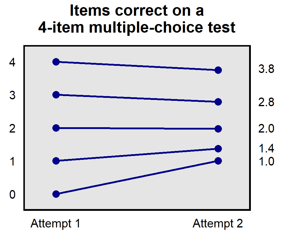
At the other end, students who got all 4 items correct on the first attempt are the 100 students who truly knew the correct response for all 4 items and are some of the students who did not truly know all 4 items but were lucky guessers: about 25 students who truly knew the correct response to 3 items correctly guessed at the 1 item that they did not know, about 6 of the students who truly knew the correct response to 2 items correctly guessed at the 2 items that they did not know, and so on. But we do not expect this lucky guessing to continue to the second attempt, as indicated in the plot above in which students who got all 4 items correct on the first attempt only got an mean score of 3.8 on the second attempt.
And in the middle of the plot, students who got 2 items correct on the first attempt had about average luck guessing and, on average, that average luck continued, so that this set of students also got about 2 items correct on the second attempt.
Sample practice items
Let’s consider a real-life example of regression toward the mean. Baseball pitchers can be evaluated on a statistic celled the Earned Run Average (ERA); lower ERAs are better, all else equal. The table below lists the ten Major League Baseball pitchers with the lowest ERAs in 1998, along with their ERA in 1999.
-----------------------------
     Player       1998  1999
      Name         ERA   ERA
-----------------------------
 Ugueth Urbina    1.30  3.69
 Trevor Hoffman   1.48  2.14
 Robb Nen         1.52  3.98
 Mike Jackson     1.55  4.06
 Graeme Lloyd     1.67  3.63
 Mariano Rivera   1.91  1.83
 John Wetterland  2.03  3.68
 Jeff Shaw        2.12  2.78
 Greg Maddux      2.22  3.57
 Kevin Brown      2.38  3.00
-----------------------------
 AVERAGE          1.82  3.24
-----------------------------
So, these ten pitchers in 1998 who had the lowest ERA had an average ERA of 1.82, but the average ERA among these ten pitchers increased to 3.24 in 1999. That’s an increase of 1.42 ERA points among these ten pitchers who had the lowest ERA in 1998. Which of the following would be your best guess about the change from 1998 to 1999 in the ERA for all pitchers in Major League Baseball?
- Less than a 1.42-point ERA increase
- About a 1.42-point ERA increase
- More than a 1.42-point ERA increase
Answer
- Less than a 1.42-point ERA increase
The overall ERA was 4.39 in 1998 among all pitchers in Major League Baseball and was 4.43 in 1999 (https://www.baseball-reference.com/leagues/MLB/pitch.shtml), so that’s only an increase of 0.04 ERA points. Here is the reason why the increase was much lower among the ten pitchers in 1998 who had the lowest ERA. For any pitcher, their ERA is some combination of skill and luck, with luck including things like getting hurt, which batters they face, what the weather is like when they pitch, how well they slept the night before, and that sort of thing. How does a pitcher get to have one of the lowest ERAs in a given year? Probably through some combination of good pitching ability and good luck. This good pitching ability will plausibly continue in the following year, but we would expect the good luck to revert back to average luck. So the list of the ten “lowest ERA” pitchers in 1998 include some great pitchers (such as Mariano Rivera) and some not-so-great pitchers who seemed to have really good luck in 1998 (such as Graeme Lloyd, who had a 1.67 ERA in 1996, but for his other years in Major League Baseball had ERAs of 2.83, 5.17, 4.50, 4.29, 2.82, 17.47, 3.31, 3.63, 4.35, 5.21, 5.87, 4.44, 5.29, 3.31, and 10.95.)
Suppose that each student in a 1,000-student course takes a test that has 10 true-false items. Each student responds to each item on this first test, but some students do not get any of the 10 items correct. Therefore, the instructor of the course requires these students to attend a study session. Each of these “zero correct” students attends the study session and then, on the second test (which has 6 different true-false items that are just as difficult as the 6 items on the first test), these students get an average of 5 items correct, so that these students raised their percentage correct from 0% to 50%. Explain why, without other evidence, this increase from 0% correct to 50% correct should not be interpreted to be due to the study session.
Answer
We would expect these “zero correct” students to get about 50% of the items correct on the second true-false test merely by guessing. A more plausible explanation for the increase from 0% correct to 50% correct is that these students were very unlucky on the first test, but that this bad luck did not continue to the second test.11.5 Ecological fallacy
The ecological fallacy is attributing characteristics of a group to individuals who are in the group. For example, cities with a large number of immigrants might have higher literacy rates than cities with a small number of immigrants, so someone might conclude that immigrants have higher literacy rates than the native population has. However, this association might merely be due to immigrants moving to places that have higher literacy rates.
11.6 Simpson’s paradox
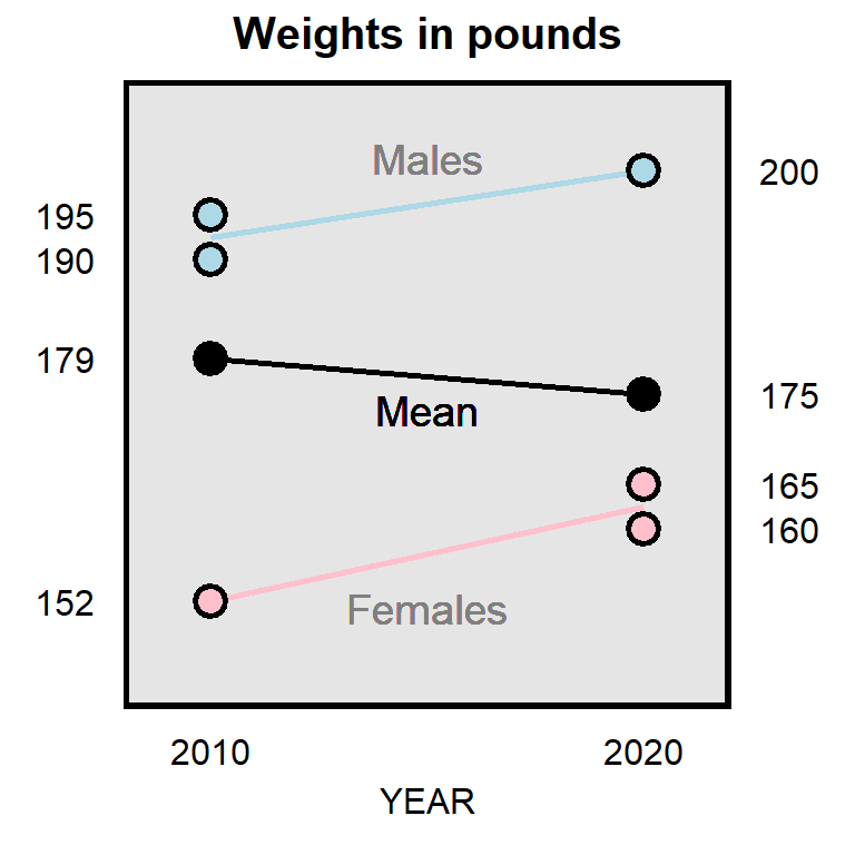
Simpson’s paradox refers to the fact that a pattern can appear in each subgroup but not appear when the subgroups are combined.
For example, it’s possible that, over the past 10 years, the mean weight among male physics majors increased, the mean weight among female physics majors increased, but that the overall mean weight among physics majors decreased. Let’s imagine that there were three physics majors in 2010 and three physics majors in 2020, with weights in the plot below.
11.7 Heterogenous effects
Heterogeneous effects are effects that differ by subgroup, such as if, in a randomized experiment testing for gender bias in candidate preference, Democrats are biased in favor of the female candidate, Republicans are biased in favor of the male candidate. A concern with heterogeneous effects is that the effects offset each other and thus produce an incorrect inference. For example, if, over the full sample, the female candidate is just as likely to be selected as the male candidate is to be selected, we might incorrectly infer that the sample had no gender bias.
Heterogeneous effects can produce overestimates or underestimates of an average effect, depending on whether the sample is representative of the population. For example, suppose that the average effect is +8 among men and is +2 among women. If men and women are equally represented in the population, then the average effect among the population will be +5, which is halfway between +8 and +2. But if men are over-represented in the sample, then the estimated average effect will be larger than the true average effect. And if women are over-represented in the sample, then the estimated average effect will be smaller than the true average effect.
11.8 Participant effects
Participants in a survey sometimes don’t pay attention and might randomly select a response. Researchers can identify respondents who don’t pay attention, by using an attention check such as:
For the next item, no matter what, select “strongly agree”.
For research involving experimental treatments, researchers can use a manipulation check to identify respondents who did not properly receive the treatment. For instance, if the experimental manipulation is the race of a target, then researchers can ask respondents to identify the race of the target that the respondent was asked about. Another type of manipulation check can measure the extent to which a treatment worked. For instance, suppose that we are assessing the influence of happiness on political attitudes, in which the research design for the treatment groups is to instruct a random set of participants to think about something happy and to then ask all participants questions about politics. To check whether participants in the “happy” group are truly more happy than participants in the control group, we might, at the end of the experiment, ask all participants to rate their happiness on a scale from 0 to 10, and then we can check whether the “happy” group has a higher mean level of happiness than the control group has.
Attention checks and manipulation checks are especially useful for assessing the value of a null result in which the analysis does not provide sufficient evidence that a treatment has an effect. In such cases, if a large percentage of participants pass each attention check and if the manipulation check indicates that participants sufficiently received the treatment, then we can credibly conclude that the null result was not due to participant lack of attention. However, if a large percentage of participants fail attention check and/or if the manipulation check indicates that participants did not sufficiently receive the treatment, then the null result should not be interpreted as indicating much about the effect of the treatment.
Let’s discuss three other participant effects:
A demand effect refers to the phenomenon in which a participant’s responses are influenced by what the participant perceives the purpose of the study to be. The bias in a demand effect depends on the participant and the study. For example, if participants think that a researcher is trying to find an association between racial bias and support for Donald Trump, then some participants might insincerely respond in a way to help the researcher find that association, and other participants might insincerely respond in a way to make it harder for the researcher to find that association.
Social desirability is when a participant does not indicate the truth, either by not responding to an item or by providing false information. Such social desirability is a particular concern for measurement of sensitive information, such as a participant’s income or the participant’s level of racism or sexism or a participant’s attitudes about contentious political issues.
Acquiescence bias is the phenomenon that, regardless of the content, some participants are more likely to agree with a statement than to disagree with a statement. Imagine a person who doesn’t care much about Social Security: if that person were asked whether they agree that funding for Social Security should be cut, then that person might agree; but if the same person were asked whether they agree that funding for Social Security should be increased, then that person might also agree. So how a statement is phrased can influence the percentage of participants that agrees with the statement, with the expectation that the percentage of “agree” responses is biased higher than it should be.
11.9 Lack of external validity
Major learning objective(s) for this section:
- Discuss the internal validity and external validity of a research design.
Validity is the extent to which a measuring tool measures what the tool is supposed to measure. Internal validity refers to the correctness of a study regarding the sample. External validity refers to the ability to generalize the sample results to a wider population, to a wider range of topics, or to the real world.
For example, suppose that we have students play a first-person shooter game in which they are instructed to shoot only targets who are holding a weapon, and in which the experiment randomizes the race of the targets so that the race of the target is randomly Black or White. The randomization of the race of the target can help us validly conclude whether the participants are racially biased in the way that they played the game. So the game will have a high amount of internal validity for assessing participant racial bias in playing the game. But even if we find evidence of racial bias among our student participants, we cannot credibly generalize that result to police officers, because students are a lot different from police officers, such as the students’ lack of training. And even if the participants were police officers, we could not credibly generalize the video game results to the real world because playing a video game is a lot different than what police officers face in reality. So the game will have a low amount of external validity for assessing racial bias among police officers in the real world.
For an example of a study with high internal validity and high external validity, researchers can conduct an audit study, such as randomly submitting resumes to employers, in which the name on the resume is either a stereotypically Black name or a stereotypically White name. The resumes are identical except for the name on the resume. The researchers then assess whether the resumes with a stereotypically Black name receive a different number of callbacks than the resumes with a stereotypically White name. This study has high internal validity because of the random assignment of names to employers, and the study has high external validity because this is very close (identical, even) to ways that people are called for interviews in the real world.
But even these audit studies aren’t perfect. One concern with resume audit study experiments is that a difference in callback rates by race could be due to social class instead of race, if, for instance, employers are less likely to call back (stereotypically Black) Jamal than (stereotypically White) Brad, but the employers might have been equally likely to call back (stereotypically Black) Jamal and (stereotypically White) Billy Bob. Moreover, audit studies can overestimate racial bias in a job market. Some audit studies match Black applicants and White applicants on all relevant factors such as education and work history that an employer might fairly consider, so that the the employer’s decision will be based on a single factor – race – and not on the potential multitude of factors such as applicant education and work history that employers might typically use in their hiring decisions.
Sample practice items
Validity refers to the extent to which a measuring tool…
- measures what the tool is supposed to measure
- produces statistically significant results
- produces consistent results
Answer
- measures what the tool is supposed to measure
Which type of validity concerns the ability to make correct claims about the sample?
- internal validity
- external validity
Answer
- internal validity
Which type of validity concerns the ability of a research result to generalize to the population?
- internal validity
- external validity
Answer
- external validity
Suppose that you are representing a corporation in a lawsuit. The plaintiff’s lawyer presents a study indicating that people who have been exposed to the corporation’s chemical have been more likely to have been diagnosed as having leukemia (p<0.05). The corporation presents a large-sample random experiment of rats that does not find sufficient evidence of a link between leukemia and exposure to the chemical (p=0.60). You could argue to the jury that the rat study should be preferred to the other study, because the rat study has…
- higher external validity
- higher internal validity
Answer
- higher internal validity
The rat study is a randomized experiment and thus permits strong causal inference. Rats differ from humans, so the rat study has low external validity.
Some research has used a first-person shooter game to measure racial bias among police officers. In the game, targets are randomly assigned to be Black or White and to be holding a weapon or holding something else like a soda can. The police officers playing the game are instructed to shoot targets who are holding a weapon and to not shoot targets who are holding something other than a weapon, and to make this decision within the short amount of time provided to make this decision. This type of study has…
- higher external validity
- higher internal validity
Answer
- higher internal validity
Suppose that a researcher finds that, for head-to-head elections in which one major party candidate was a man and the other major party candidate was a woman, the woman candidate in the election was on average less likely to win election than was the man candidate was (p<0.05). Does this analysis have a high amount of internal validity for assessing whether sexism against women caused these women candidates to have been less likely to be elected than the men candidates were?
- Yes, because these are data from real elections
- Yes, because the p-value was less than p=0.05
- No, because there are plausible alternate explanations that the analysis did not address
- No, because the analysis should have included all elections, and not only elections in which one major party candidate was a man and the other major party candidate was a woman
Answer
- No, because there are plausible alternate explanations that the analysis did not address
Suppose that, for a set of job openings posted online, researchers send one resume to each opening. The resume is the same for all openings, except that the first name on the resume is randomly assigned to be either a male name or a female name. Researchers then compare the percentage of callbacks that the “male” resume received compared to the percentage of callbacks that the “female” resume received. Does this analysis have a high amount of internal validity for assessing whether gender bias influenced the callback rate?
- Yes
- No
Answer
- Yes
Suppose that a researcher tests for racial bias. The researcher conducts a randomized experiment in which a large sample of students from the local college are randomly given a story about a Black man convicted of a DUI or a White man convicted of a DUI. The researcher analyzes the responses to see whether there is a difference between the mean sentence length recommended for the Black man convicted of a DUI and the mean sentence length recommended for the White man convicted of a DUI. Does the study have a high amount of internal validity and/or a high amount of external validity?
Answer
The study has a high amount of internal validity, because the study is a randomized experiment that manipulated only the man’s race. but the study does not have a high amount of external validity, because college students are plausibly not representative of persons in the legal system who will decide in real life the sentence length for a DUI.11.10 Researcher bias or researcher error
Major learning objective(s) for this section:
- Discuss how inferences can be biased by researcher bias and researcher error.
Sometimes researchers intentionally misrepresent data or intentionally report misleading analyses, such as researchers reporting on a misleading subset of research that they conducted. Sometimes researchers report misleading analyses merely through good faith errors, in which the researchers do not appreciate the fact that their analyses are misleading. Below are some examples of how research might be misleading, incorrect, or otherwise flawed or potentially flawed.
Researcher flexibility: Selective reporting
From Hartnett and Haver 2022:
With 40% of Trump voters in our study stating that Trump should resist the election results even in a scenario in which Biden won by a large popular-vote margin, the precedent of a peaceful transfer of power in American elections was shaken even before the election.
Hartnett and Haver 2022 did not report the corresponding “resist” percentage among Biden voters, so that we as readers do not know if Trump voters are distinctive in wanting their candidate to resist the election results if their candidate lost. Did the researchers not measure this “resist” percentage among Biden voters, or did the researchers measure this “resist” percentage and then decide to not report the results? Check for hidden text in the final few pages of their codebook, referenced in this tweet.
Researcher flexibility: Selective predictors
Researchers might include a biased selection of predictors. For example, as indicted in the plot below, in the contemporary United States, Republican partisanship is associated with more negative ratings about Blacks, Hispanics, and Asians, and Democratic partisanship is associated with more negative ratings about Whites.

Political science research about racial attitudes often does not include measures of negative attitudes about Whites. For example, Graham et al 2021 “Who wears the MAGA hat? Racial beliefs and faith in Trump” includes measures that permit participants to report negative attitudes about Blacks and to report negative attitudes about Hispanics, but does not permit participants to report negative attitudes about Whites. Each of these predictors is a plausible explanation for the decision to wear or not wear a “Make America Great Again” hat in public, but negative attitudes about Whites is also a plausible explanation that Graham et al 2021 did not include.
Researcher flexibility: Selective measures of misinformation
Selection of items is particularly important for research attempting to determine which groups are most misinformed. For example, Abrajano and Lajevardi 2021 reported that:
We find that White Americans, men, the racially resentful, Republicans, and those who turn to Fox and Breitbart for news strongly predict misinformation about [socially marginalized] social groups.
The concern with an inference like this is the extent to which the inference is merely due to a biased selection of misinformation measures. In the United States, more positive attitudes about socially marginalized groups associates with being a Democrat relative to being a Republican, so Democrats will plausibly be misinformed in a way that favors socially marginalized groups, and Republicans will plausibly be misinformed in a way that disfavors socially marginalized groups.
For example, one of the misinformation items from Abrajano and Lajevardi 2021 is “Most terrorist incidents on US soil have been conducted by Muslims”. The only misinformation that this item can detect is Muslim terrorism being perceived to be more common than it actually is, and this type of misinformation is plausibly more common among Republicans. Abrajano and Lajevardi 2021 did not include an item that permits identification of the misperception that Muslim terrorism is less common than it actually is, which is a type of misinformation that is plausibly more common among Democrats. For example, data from the National Consortium for the Study of Terrorism and Responses to Terrorism at the University of Maryland, College Park, seems indicates that, in the 21st century, Muslim terrorists have killed more Americans than other terrorists, given that the vast majority of Americans killed by terrorists were killed in the 9/11 attacks. Therefore, on at least this misinformation item, the Abrajano and Lajevardi 2021 research design was plausibly biased in favor of the inference that misinformation is more common among Republicans than among Democrats.
Researcher flexibility: Disputed terms
Another potential flaw involves definition of disputed terms, such as racism and sexism. Consider one of the items that Knuckey 2018 used to measure modern sexism:
Should the news media pay more attention to discrimination against women, less attention, or the same amount of attention they have been paying lately?
Potential responses include “A great deal more attention”, “Somewhat more attention”, “A little more attention”, “Same amount of attention”, “A little less attention”, “Somewhat less attention”, and “A great deal less attention”. To be coded at the non-sexist end of the measure of modern sexism, a participant must agree that the news media should pay a great deal more attention to discrimination against women. But it seems possible for a non-sexist participant to think that the news media is currently paying enough attention to discrimination against women.
Or consider the item below, which is one of two items that Knuckey 2018 used to measure traditional sexism:
Do you think it is easier, harder, or neither easier nor harder for mothers who work outside the home to establish a warm and secure relationship with their children than it is for mothers who stay at home?
Response options for this item ranged from “A great deal easier” to “A great deal harder”. From what I can tell, to be coded at the non-sexist end of the scale, a participant must agree that establishing a warm and secure relationship with their children is easier for mothers who work outside the home than for mothers who stay at home. I can’t see why it would be sexist to expect that spending more time with a child will make it easier to establish a warm and secure relationship with the child, but the non-sexist end of the scale for the Knuckey 2018 coding of this item requires you to believe the opposite.
Researcher flexibility: Incorrect use of unipolar measures
Many measures avoid particular attitudes. For example, people can prefer their ingroup to an outgroup (ethnocentrism), prefer the outgroup to their ingroup (xenocentrism), or be neutral between their ingroup and an outgroup (neither ethnocentrism nor xenocentrism). But check how Allen and Lindsay 2023 coded their measure of ethnocentrism:
Respondents. evaluation of whites, their own racial group, are subsequently subtracted from their ratings of other groups and aggregated on a continuous scale, with zero being the least ethnocentric and one being the most ethnocentric. A hypothetical score of zero indicates that group members rate other groups as highly superior to their own, a score of 0.5 indicates that members rate their own group equal to all other groups, and a score of 1 indicates that group members rate their own group as superior to all other groups.
Thus, for Allen and Lindsay 2023, a participant rating their group equal to other groups is merely moderate ethnocentrism, at 0.5 on the 0-to-1 ethnocentrism scale, even though rating your group equal to other groups is not preferencing your group in any way. Low ethnocentrism on the Allen and Lindsay 2023measure isn’t zero ethnocentrism: it’s negative ethnocentrism.
Researcher omission of relevant controls
Peay and McNair 2021 reported on a study suggesting that the number of Black Lives Matter protests in a state influenced policy changes in that state:
Are states with more protests more active in passing police reforms?…Each of the models in Table 1 evaluates the relationship between the number of BLM protests in a given state and the total number of reformative policies adopted similarly. In all three models, we find a statistically significant, positive influence…
So states that have a larger number of Black Lives Matter protests pass a larger number of police reforms. But maybe the association is merely due to population size, in which larger population states have a larger number of protests (due to having a larger population) and pass a larger number of laws of any type (due to having a larger population). I checked if this was plausible, by analyzing whether the number of BLM protests in a state predicted the number of childhood obesity laws passed by a state. The predictive power of BLM protests was about the same, no matter whether the outcome was police reform laws or childhood obesity laws.
Sample practice items
On climate.gov, Lindsey and Dahlman (2022) indicates that the mean surface temperature of the Earth has increased by about 2°F since 1880. Suppose that a large representative sample of Democrats and a large representative sample of Republicans are asked to indicate the correct response to the item: “Has the mean surface temperature of the Earth increased since 1880?”. Results indicate that the percentage of Democrats who correctly respond “Yes” is higher than the percentage of Republicans who correctly respond “Yes”, with a p-value of p<0.05 for a test of the null hypothesis that these percentages equal each other.
Does this analysis contain sufficient evidence to conclude, at the conventional level in political science, that, at least on average, a higher percentage of Republicans are misinformed about how much the mean surface temperature of the Earth has increased since 1880, compared to the percentage of Democrats who are misinformed about how much the mean surface temperature of the Earth has increased since 1880?
- Yes
- No
Answer
- No