2 Sampling

2.1 Sampling error

Major learning objective(s) for this section:

Identify the sample and the population for a particular study.

A population is the set of things of interest for a study. A sample is the set of things that were studied for the study. For example, suppose that we are interested in the percentage of U.S. residents who approve of the U.S. president, but we survey only students in this POL 138 course. In this case, U.S. residents are the population, and students in this POL 138 course are our sample of that population.

The difference between the sample and the population is sampling error. This isn’t necessarily error in the sense of a mistake, but this error in the sense of an imperfection.

Sample practice items

Suppose that a researcher is interested in the percentage of Illinois residents that will vote in the next election. The researcher surveys 1,000 randomly selected Illinois residents. What is the sample of this study?

Illinois residents
the 1,000 randomly selected Illinois residents selected for the survey

Answer

the 1,000 randomly selected Illinois residents who were surveyed

Illinois residents
the 1,000 randomly selected Illinois residents who were surveyed

Answer

Illinois residents

2.2 Law of Large Numbers

Major learning objective(s) for this section:

Explain the benefit of random sampling from a population.
Know the implications of the Law of Large Numbers.

In a random sample of a population, each member of the population has an equal chance of being sampled. The benefit of this random sampling is that it tends to produce samples that have characteristics that are close to matching the characteristics of the population, especially if the sample is large. The Law of Large Numbers is that, as the number of randomly selected observations in a sample increases, the characteristics of the sample will tend to approach the characteristics of the population.

Let’s run a simulation to illustrate this. The population will be the set of whole numbers from 0 through 200, so the mean of the population is 100. The simulation will randomly draw numbers from this population and will calculate the mean of the sampled numbers. Some of the samples will be small (such as 2 or 3 sampled numbers) and some of the samples will be large (such as 100 or 200 sampled numbers). As the plot below indicates, compared to the means for the smaller samples, the means for the larger samples tend to be closer to the population mean of 100.

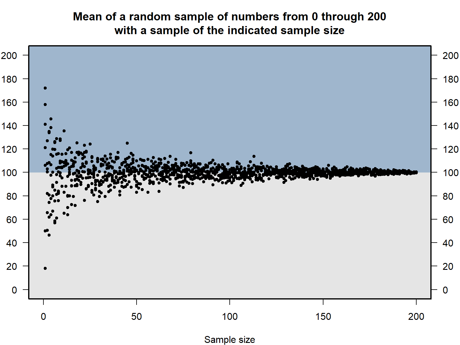
Because of the Law of Large Numbers, the mean of a smaller random sample is more likely to be extremely far from the mean of the population, compared to the distance that the mean of a larger random sample is from the mean of the population. Flip a fair coin twice, and half of the outcomes are expected to be the most extreme percentages possible (0% heads, and 100% heads). But flip a fair coin six times, and these extreme percentages of 0% heads and 100% heads occur only 2 times in 64 possible outcomes, which is about 3% of the time. Smaller random sample sizes are not expected to bias the mean of the sample to be necessarily higher or necessarily lower than the mean of the population. But, compared to the mean of a larger random sample, the mean of a smaller random sample is expected to be farther from the mean of the population.

The fact that extreme means are more likely to occur in smaller random samples than to occur in larger random samples has implications for the real world. For example, on average, we would expect that the Illinois county with the highest cancer rate is, all else equal, more likely to be a small population county than to be a large population county, even if nothing in these Illinois counties is causing variation in cancer rates. Moreover, all else equal, we would expect that the Illinois county with the lowest cancer rate is more likely to be a small population county than to be a large population county, even if nothing in these Illinois counties is causing variation in cancer rates.

Sample practice items

Amy and Bob are political science majors who are estimating the mean height of students at Faber College. Amy randomly selects 200 students at Faber College, measures their heights, and calculates the mean height among these students. Bob instead visits all four sections of a POL 100 class, measures the heights of all 400 students in these sections, and calculates the mean height among these students. Who has the more credible estimate of the mean height of students at Faber College?

Amy, because her sample size is smaller
Amy, because she used a random sample
Bob, because his sample size is larger
Bob, because his sample included all students in POL 100

Answer

Amy, because she used a random sample

Suppose that 40% of a population of students is male. Which of the following is more likely to produce a sample that is 40% male?

a random sample of 40 students
a random sample of 200 students

Answer

a random sample of 200 students

Suppose that a school randomly assigns students to a small class of 10 students or to a large class of 50 students, so that half of classes are small and half of classes are large. Each student takes a multiple-choice test, and the school calculates the mean score on this test for each class. Which would be expected about the class with the highest mean score on the test?

It is a small class.
It is a large class.
It is just as likely to be a small class as a large class.

Answer

It is a small class.
Smaller samples are more likely to have an extreme mean.

It is a small class.
It is a large class.
It is just as likely to be a small class as a large class.

Answer

It is a small class.
Smaller samples are more likely to have an extreme mean.

Suppose that Amy asks a random 10 ISU students to randomly pick one number from 0 to 100, and Bob asks a random 500 ISU students to randomly pick one number from 0 to 100. Amy calculates the mean from her sample, and Bob calculates the mean from his sample. Select all of the following, if any, that should be expected:

Amy’s mean is higher than Bob’s mean.
Amy’s mean is lower than Bob’s mean.
Compared to Bob’s mean, Amy’s mean is closer to 50.
Compared to Bob’s mean, Amy’s mean is farther from 50.

Answer

Compared to Bob’s mean, Amy’s mean is farther from 50.
Smaller samples are more likely to have an extreme mean. So, compared to Bob’s mean, Amy’s mean should be expected to be farther from 50 than is Bob’s mean. But there is no reason to expect Amy’s mean to be higher or lower than Bob’s mean.

2.3 Imbalanced sample sizes

All else equal, larger random samples are better than smaller random samples, because larger random samples provide more precision for our estimates. Compared to the mean of a larger random sample, the mean a smaller random sample is expected to be farther from the true population mean, but the mean of a smaller random sample is not expected to be biased higher or lower than the true population mean.

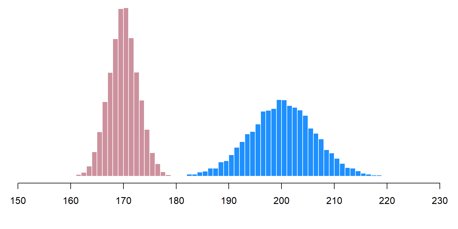
Because of this, if two groups are being compared to each other, a difference in the sample sizes of the groups will not bias the comparison. Suppose that we are estimating the gender gap between the mean weight of female U.S. residents and the mean weight of male U.S. residents. Having a larger sample of females and a smaller sample of males won’t bias the estimate of the gender gap in mean weights to be lower than or higher than the true gender gap. The imbalance in the sample sizes in this case merely means that the estimate of the mean weight for females will likely be more precise than the estimate of the mean weight for males, as indicated in the plot below, based on random samples of 25 females from a female population with a mean weight of 170 pounds and random samples of 5 from a male population with a mean weight of 200 pounds. Due to this difference in sample size, the distribution of weights for the female samples is thinner than the distribution of weights for the male samples; but the difference in sample sizes does not bias the estimate of the gender gap in mean weights across the samples to be lower than or higher the true gender gap in mean weights.

Sample practice items

Amy and Bob are political science majors who are estimating the size of the gender gap among Faber College students in support for the president of Faber College. Amy has a random sample of 40 female Faber College students and a random sample of 80 male Faber College students. Bob has a random sample of 30 female Faber College students and a random sample of 30 male Faber College students. Whose data will provide the best estimate of the size of the gender gap among Faber College students in support for the president of Faber College?

Answer

Amy. The difference in sample size won’t be expected to bias Amy’s estimate of the gap. The larger sample sizes for Amy compared to Bob means that Amy will likely have the more precise estimate of the gender gap, without any loss in accuracy relative to Bob.

2.4 Relatively small samples can be useful

Let’s run a few simulations to show that, even with a large population, characteristics of relatively small random samples can be expected to be relatively close to the characteristics of the population. Let’s use a population that has 100 million people, of whom 60 million are female and 40 million are male, for a population that is 60% female and 40% male. This first simulation randomly samples 100 of the 100 million people and calculates the percentage of the sample that is female. I’ll run the simulation 5,000 times and plot the percentage female for each of the 5,000 samples:

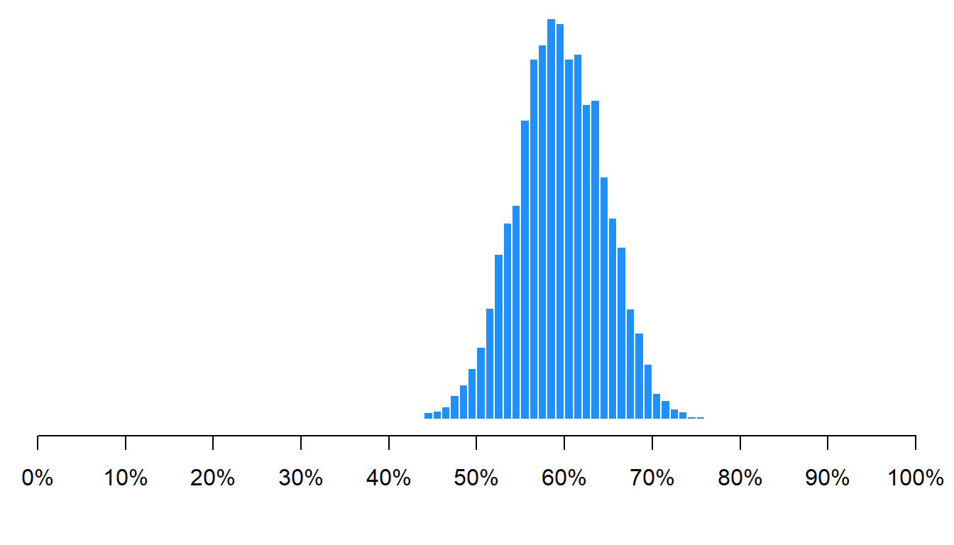
As indicated in the histogram above, the mean percentage female across all samples was 60%, which is the correct percentage female in the population. Not all samples had a percentage female that was exactly 60%, but 95% of the percentage females in the 5,000 simulated samples fell between 50% female and 70% female.

Let’s run the same simulation, but instead of randomly sampling 100 of the 100 million people each time, let’s randomly sample 250 of the 100 million people each time:

As indicated in the histogram above, the mean percentage female across all samples was 60%, which is the correct percentage female in the population. Not all samples had a percentage female of exactly 60%, but 95% of the percentage females fell between 54% female and 66% female. That’s not too bad, for sampling only 250 people from a population of 100 million.

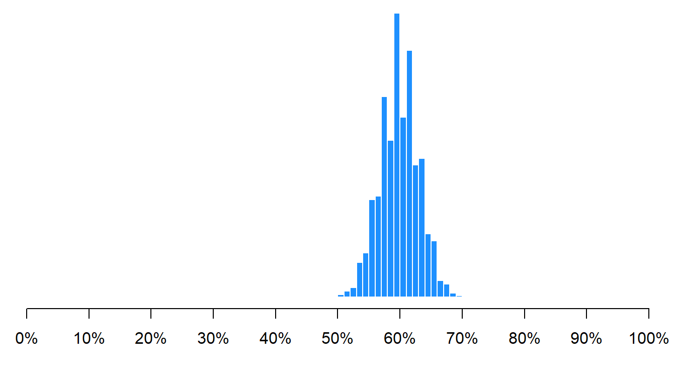
Let’s run the same simulation, but let’s randomly sample 1,000 of the 100 million people each time:

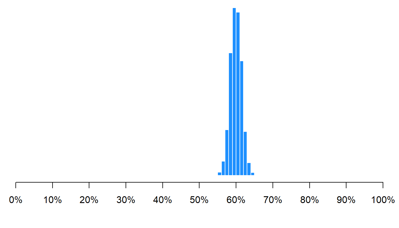
As indicated in the histogram above, the mean percentage female across all samples was 60%, which is the correct percentage female in the population. Not all samples had a percentage female of exactly 60%, but 95% of the percentage females fell between about 57% female and 63% female. That’s not too bad, for sampling only 1,000 people from a population of 100 million.

2.5 Sampling weights

Major learning objective(s) for this section:

Explain why researchers weight survey data.
Calculate and apply weights to address selection bias into a sample.

The Law of Large Numbers indicates that a larger random sample will on average be expected to produce a more accurate estimate of the population, compared to the estimate that is produced by a smaller random sample. However, the Law of Large Numbers does not mean that a larger non-random sample will be expected to produce a more accurate estimate than a smaller non-random sample does. The key feature for the Law of Large Numbers is that the samples are random. For instance, if Fox News had a poll on their website measuring support for Republicans, results from that poll would likely not be an accurate sample of the U.S. population, even if the sample for the poll had millions of U.S residents. Persons who visit the Fox News website are plausibly more Republican on average compared to the typical U.S. resident, so the poll would likely be biased to overestimate support for Republicans.

Remember that a population is the set of things of interest for a study, and a sample is the set of things that were studied for the study. Researchers have tools to address samples that are not representative of their population on relevant characteristics. For example, about 19% of the U.S population is Hispanic, but we might have a sample in which only 11% of the sample is Hispanic. For this, we can apply sampling weights. For these weights, we can multiply each observation by a number that represents whether the observation is overrepresented, underrepresented or correctly represented in the sample. Let’s use race/ethnicity as an example, for a hypothetical sample:

	Population %	Sample %	Sampling Weight	Sampling Weight
Non-Hispanic White	61	65	61 / 65	0.938
Non-Hispanic Black	12	12	12 / 12	1.000
Hispanic	19	11	19 / 11	1.727
Non-Hispanic Asian	6	3	6 / 3	2.000
Other	2	9	2 / 6 \| 0.182 \|

The sampling weight for a group is calculated by dividing the population representation by the sample representation. For this example, Non-Hispanic Asians are 6% of the population and 3% of the sample, so the weight for each Non-Hispanic Asian in the sample would be 2, if weights were only used for race/ethnicity. We multiply each Non-Hispanic Asian observation in the sample by 2, to get the sample Non-Hispanic Asian percentage of 3% to equal the population Non-Hispanic Asian percentage of 6%.

The survey weight formula in general is:

\[\text{Survey weight}=\frac{\text{% in the population}}{\text{% in the sample}}\]

Generally speaking, if a person is underrepresented in the sample, then the sampling weight will be greater than 1, because multiplying by a number greater than 1 will increase the emphasis on that observation. And if a person is overrepresented in the sample, then the sampling weight will be less than 1, because multiplying by a number less than 1 will increase the emphasis on that observation. And if a person is correctly represented in the sample, then the sampling weight will be 1, because multiplying by 1 will not change the emphasis on that observation.

Survey weights often account for multiple factors, such as gender, race, ethnicity, education, and income. The survey weight logic applies when the weights address more than one factor. For example, if Black women are 6% of our population and are 4% of our sample, then the survey weight that gets applied to each Black women in the sample would be 6 \(\div\) 4 or 1.5.

Weights are important for getting correct estimates of population percentages, both for descriptive questions such as the percentage of U.S. residents who approve of the U.S. president, but also for causal questions, such as the extent to which a person’s personal economic condition influences that person’s support for the U.S. president. Weights for causal inference are important because causal effects sometimes differ across subsets of the population, such as if a causal effect were larger among women than among men. If, in that case, our sample oversampled women, then – if we did not apply weights – our estimate of the causal effect would plausibly be larger than the true effect in the population.

Sometimes researchers want a sample that is not representative of the population. For example, suppose that we want to assess differences in political attitudes among racial groups in the United States. If we have a representative sample of 5,000 U.S. residents, the sample might have 4,000 White U.S residents but have only 600 Black U.S residents, so that the data provide a lot less information about Black U.S residents than about White U.S. residents. We can address this by oversampling Blacks so that Blacks are, say, 26% of the sample, but then applying weights so that Blacks are closer to the Black percentage of the U.S. population, of about 13%.

Researchers can use weights to address differences between sample characteristics and population characteristics, if the sample characteristics and population characteristics are known or can be plausibly estimated. For example, if we know from U.S. Census data that about 12% of the U.S. population is Black, and we ask participants in our survey to indicate their race, then we can use weights to address any difference between the sample percentage that is Black and the population percentage that is Black.

But we sometimes don’t have good data about particular characteristics of a population. For example, we might not have good data about the percentage of the U.S. population that is a conspiracy theorist, so if conspiracy theorists are less likely to take our survey, we might misestimate characteristics of the population that are correlated with being a conspiracy theorist, because – without a good estimate about the percentage of conspiracy theorists in the population – we can’t be sure of how good our weights are for any weights that we use for conspiracy theorists.

Sample practice items

Researchers might want to weight survey data…

when the sample is too large
when the population is homogeneous
when sample characteristics do not match the population characteristics
when the p-value for a test of the null hypothesis is not less than p=0.05

Answer

when sample characteristics do not match the population characteristics

Suppose that, for a survey, 70% of the sample is female and 55% of our population is female. The survey weight applied to females in this case should be…

70/55
55/70
30/45
45/30

Answer

55/70

If the mean survey weight for a group is 0.4, then that means that the group was…

undersampled, relative to the group’s percentage of the population
oversampled, relative to the group’s percentage of the population
neither undersampled nor oversampled, relative to the group’s percentage of the population

Answer

oversampled, relative to the group’s percentage of the population
A weight of 1 does not change the group’s weight. A weight above 1 increases the group’s contribution to the population estimate, and a weight under 1 reduces the group’s contribution to the population estimate.

Suppose that men are 30% of a given population and women are 70% of a given population. Suppose also that men are 50% of our sample of the population and that women are 50% of our sample of the population. And suppose that men in our sample of the population had a mean height of 180 cm and that women in our sample of the population had a mean height of 170 cm. What would be the best estimate for the mean height of the population, assuming that the samples are representative? [Hint: This is a weighted mean question].

Answer

We are estimating the population mean height, so we can ignore the sample percentages. The problem then becomes a weighted mean problem, so:

(180cm)(0.30) + (170cm)(0.70)
       54cm     +     119cm
             173 cm

2.6 The normal distribution

Major learning objective(s) for this section:

Know how a uniform distribution can be produced.
Know how a normal distribution can be produced.
Know the rule of thumb that, for a normal distribution, about 95% of the data points fall within two standard deviations of the mean.

The shape of data when the data are plotted by frequency is referred to as a distribution. There are many different distributions, but for this course we will focus on the uniform distribution and the normal distribution.

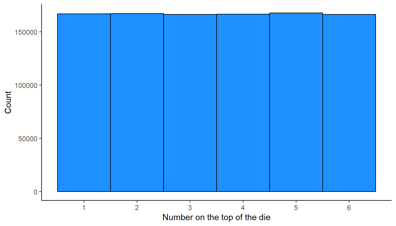
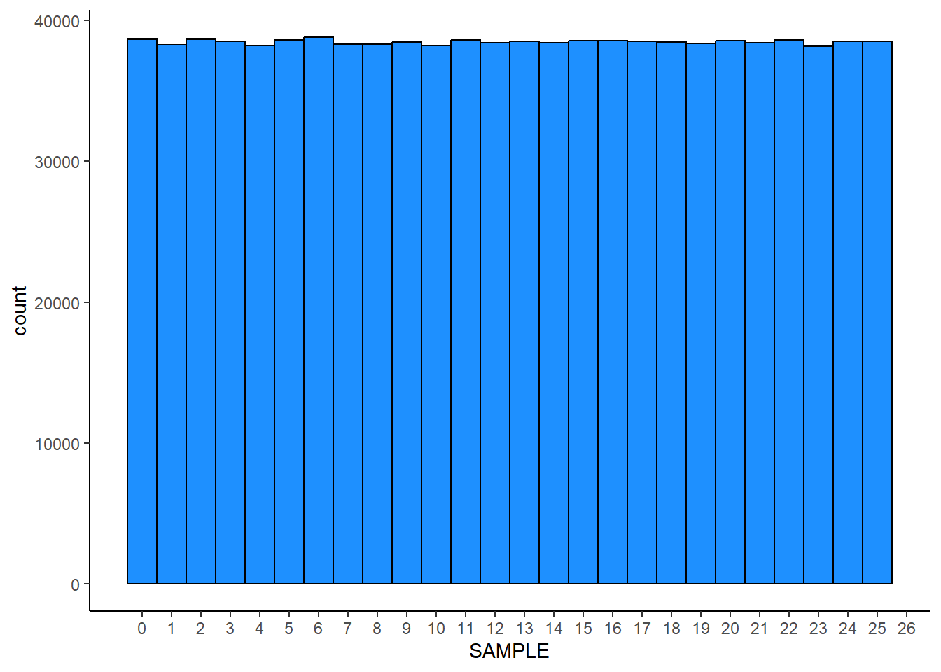
In a uniform distribution, each value has the same probability of selection, so each value is expected to occur just as frequently as any other value, with the only difference in observed frequency being due to random chance. For example, if we roll a fair six-sided die that is numbered from 1 through 6, each number on the die has the same probability of being selected, so that the distribution of values from the die will be something like the plot below, which simulates 1 million rolls of a six-sided die numbered 1 through 6.

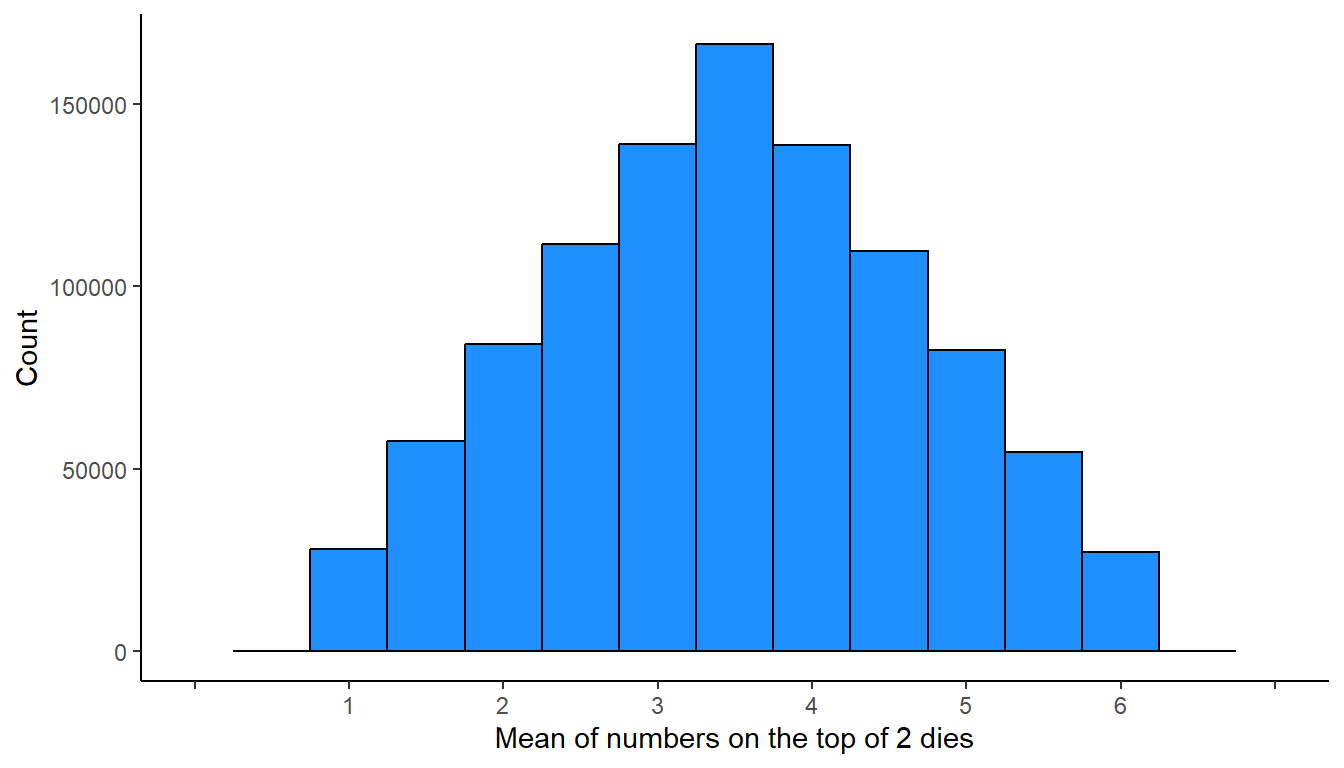
The plot below occurs if we roll two six-sided dies 1 million times, record the numbers on the top of the dies each time, calculate the mean of the two numbers, and plot the number of times that each mean appeared. The distribution of means for rolling two six-sided dies is not uniform, because all outcomes are not equally likely. For example, the only way to get a mean of 1 is to get a 1 on the first roll and a 1 on the second roll. But there are more ways to get a mean of 2 (1 and 3, 3 and 1, and 2 and 2). And even more ways to get a mean of 3.

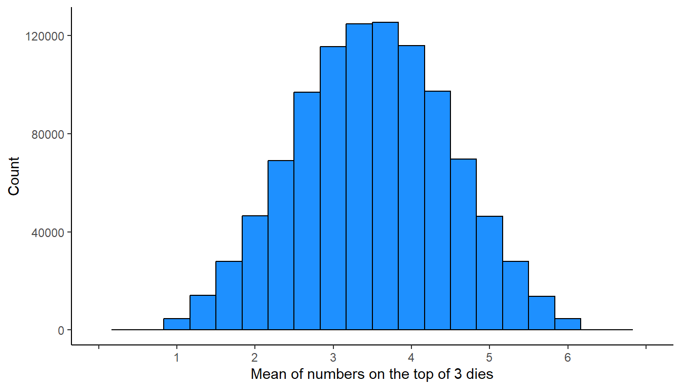
The plot below occurs if we roll three six-sided dies 1 million times, record the numbers on the top of the dies each time, calculate the mean of the three numbers, and plot the number of times that each mean appeared…

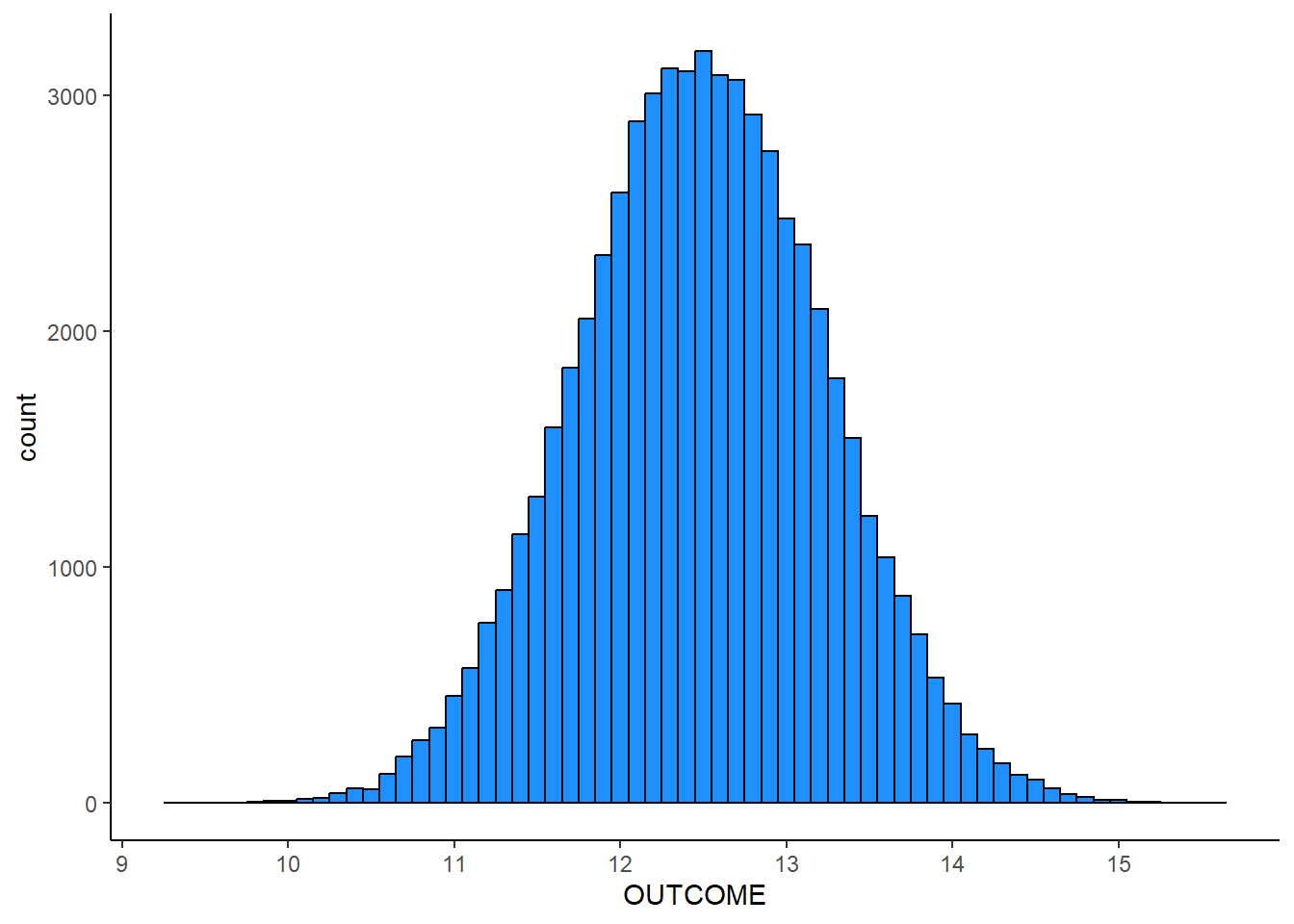
The plot below occurs if we roll ten six-sided dies 1 million times, record the numbers on the top of the dies each time, calculate the mean of the ten numbers, and plot the number of times that each mean appeared…

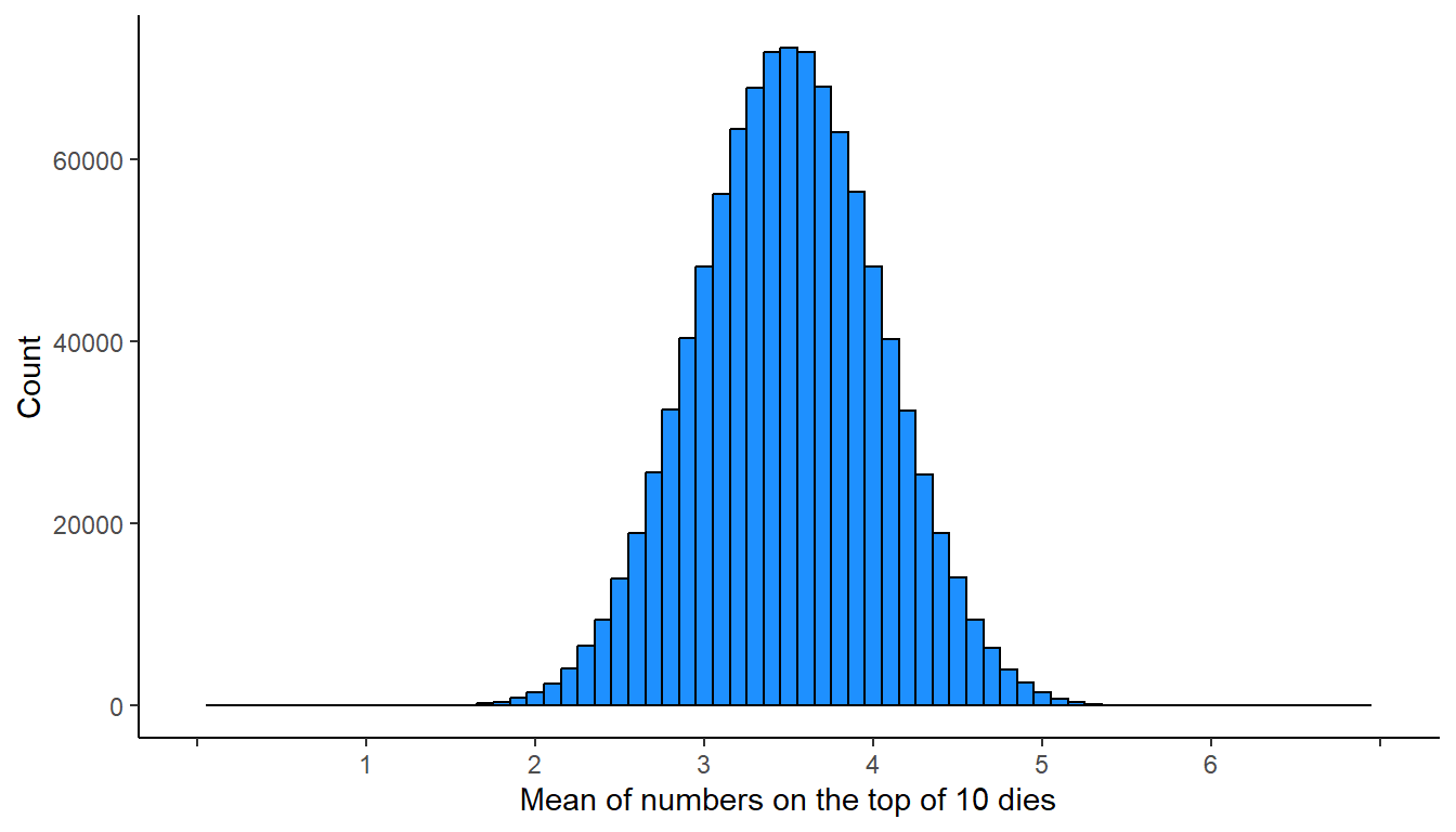
The plot above is a histogram of the values, but we can also illustrate a distribution with a curve, in which the height of the curve represents the frequency of particular values in the distribution. For instance, in the distribution below, there are about 72,000 outcomes at a mean of 3.5, about 48,000 outcomes at a mean of 3.0, and about 1,500 outcomes at a mean of 2.0.

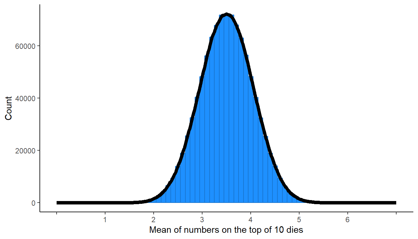
The distribution above is a normal distribution. A normal distribution has particular characteristics, such as a “bell” shape, the mean equaling the median, the left side being symmetric with the right side, and the distribution having many more observations in the middle of the distribution than at the ends of the distribution. The normal distribution (or a distribution close to the normal distribution) occurs in many real-life situations, such as people’s weights or people’s heights.

The normal distribution has the useful property that:

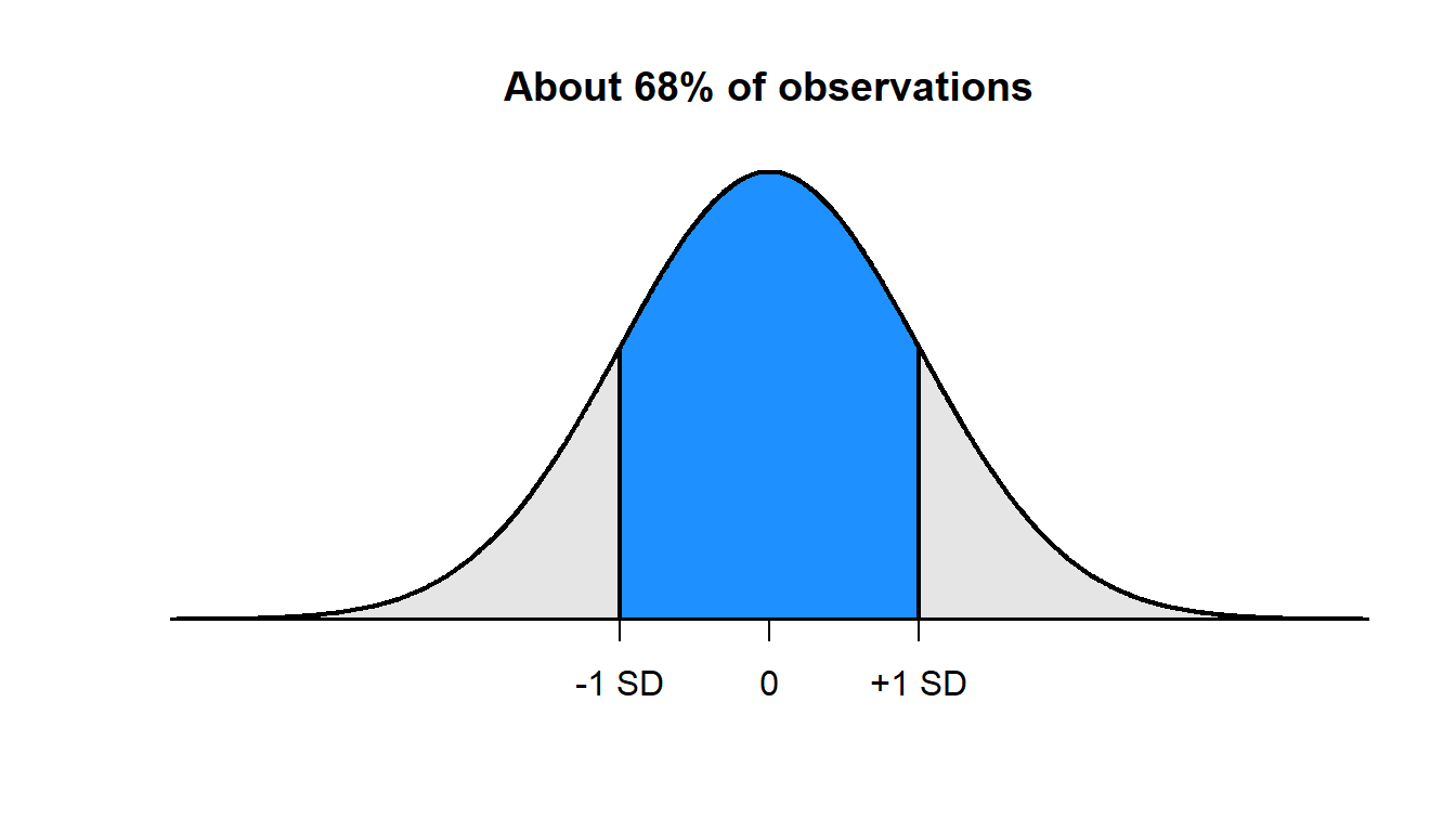
about 68% of points fall within 1 standard deviation of the mean
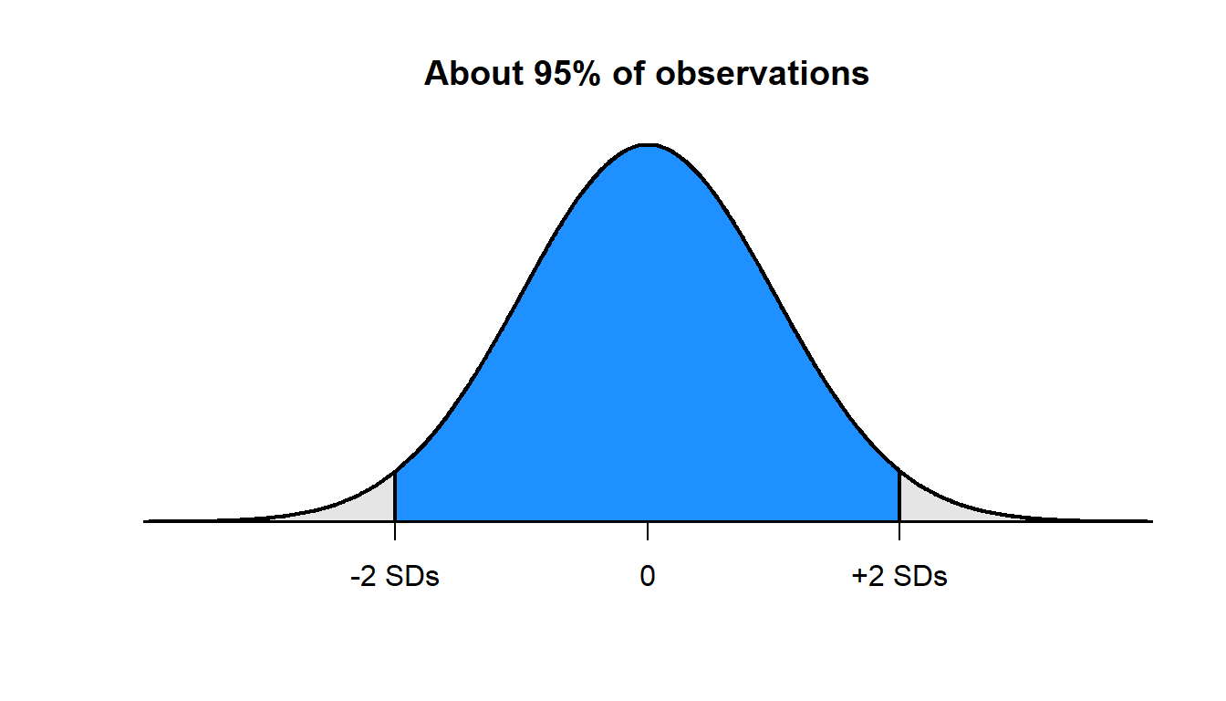
about 95% of points fall within 2 standard deviations of the mean
about 99.7% of points fall within 3 standard deviations of the mean

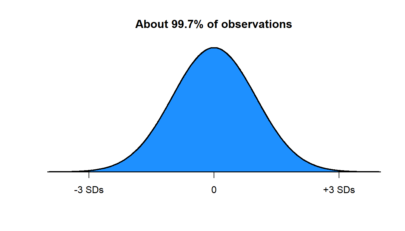
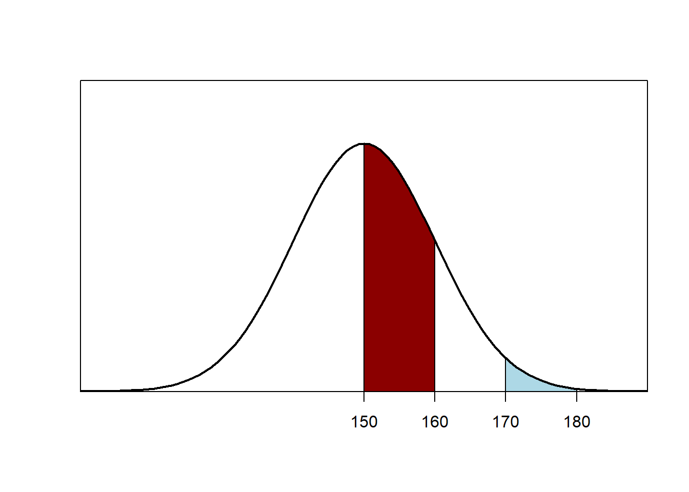
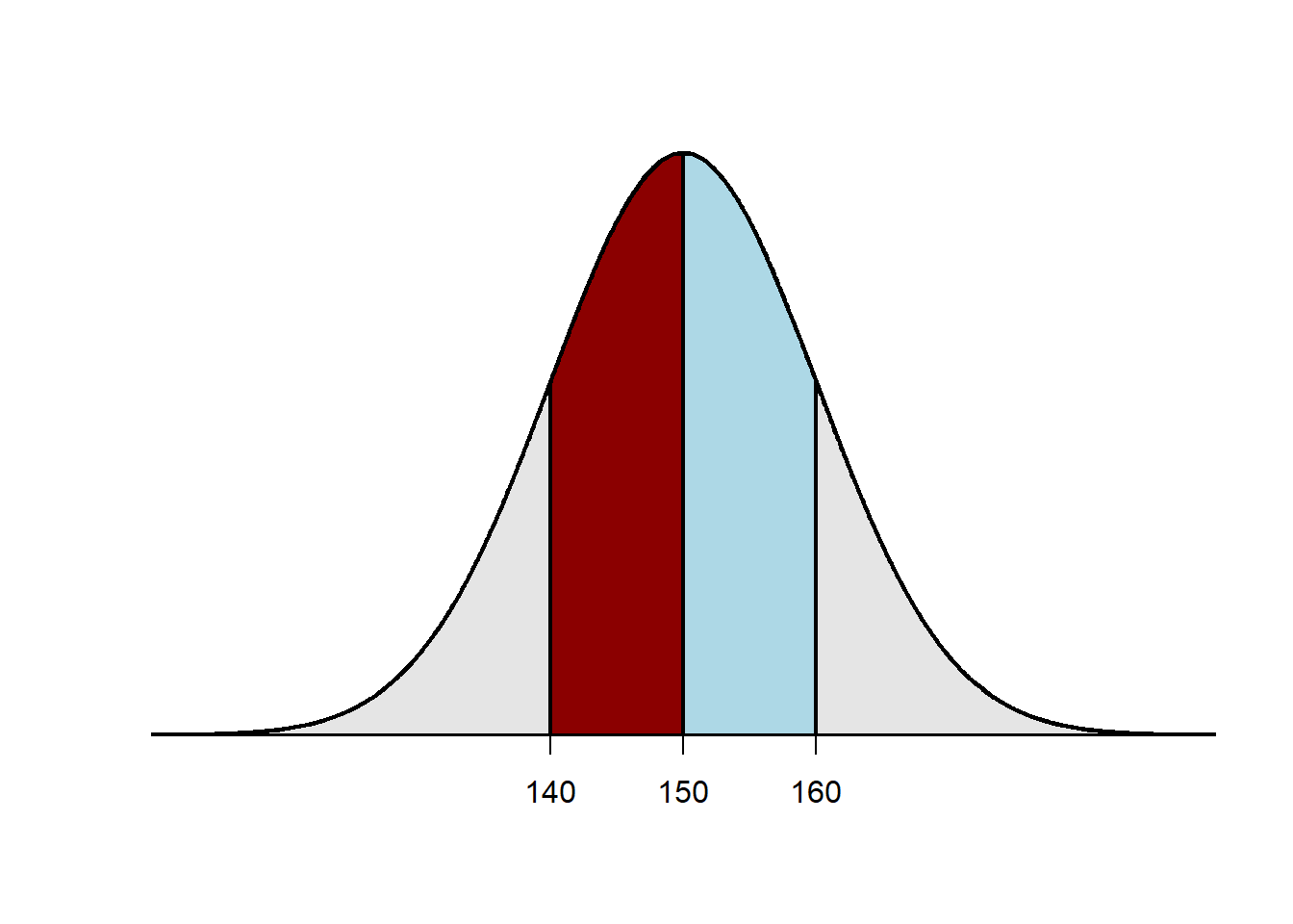
So, suppose that test scores have a mean of 150 and a standard deviation of 10 and that the test scores follow a normal distribution. If so, then:

about 68% of scores should be between 140 and 160
about 95% of scores should be between 130 and 170
about 99.7% of scores should be between 120 and 180.

Let’s, for example, consider the 95% rule above. If 95% of scores are between 130 and 170, then that leaves 5% of scores that remain, and this 5% of scores will be evenly split between the bottom of the distribution and the top of the distribution. So about 2.5% of scores will be expected to be below 130 and about 2.5% of scores will be expected to be above 170. So a score at 130 would be at about the 2.5th percentile and a score at 170 would be at about the 97.5th percentile.

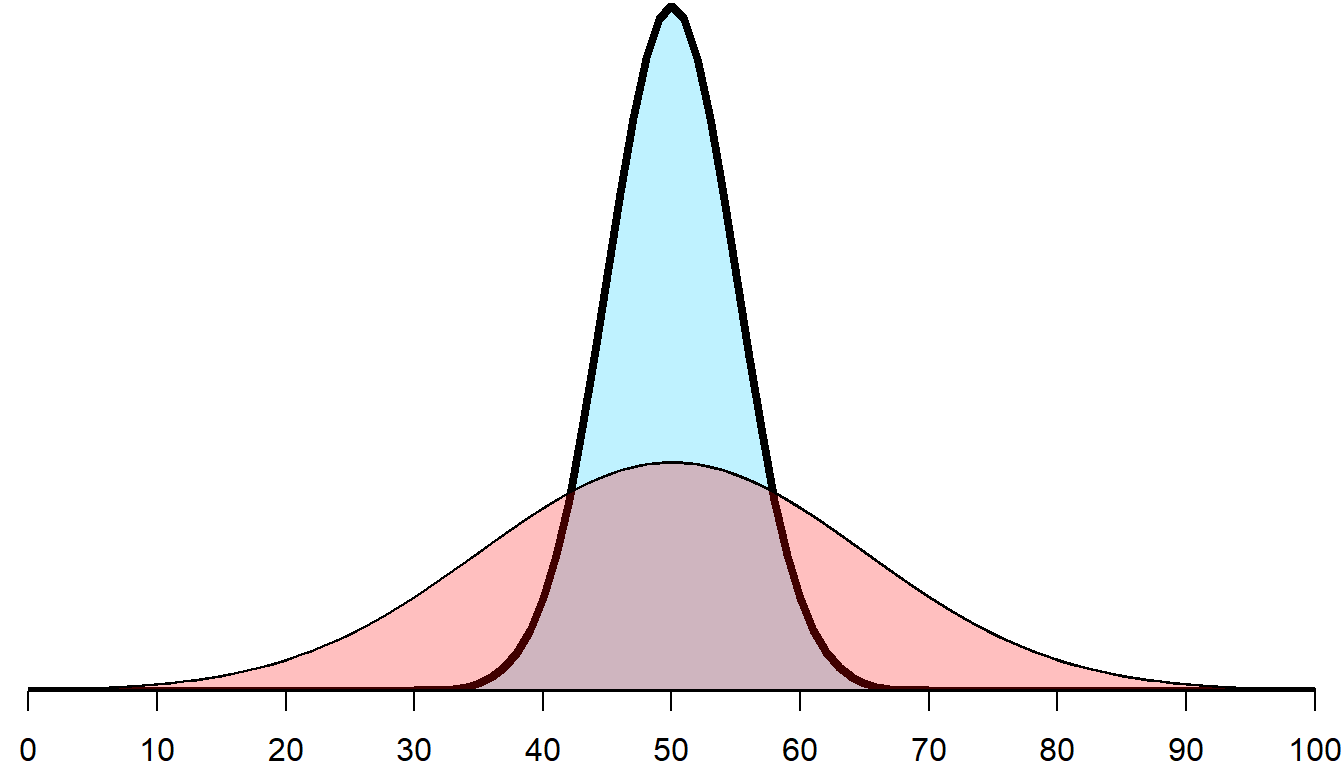
There are many different potential heights, widths, and centers of a normal distribution. Below, the standard deviation for the thick line (blue region) is 5 and the standard deviation for the thin line (pink region) is 15:

Sample practice items

The image below is an example of a…

normal distribution
uniform distribution

Answer

uniform distribution

The image below is an example of a…

normal distribution
uniform distribution

Answer

normal distribution

Suppose that each of 200 students responds to one test question written in Hungarian, in which the question has two possible options: true and false. Exactly one of these two options is correct for the question. None of the students can read Hungarian, so each student randomly guesses at the question. The distribution of student percentages correct will be more likely to look like…

a uniform distribution
a non-uniform distribution

Answer

a uniform distribution
About 50% of students will be expected to guess the correct response, and about 50% of students will be expected to guess the incorrect response, so, the percentages correct will be expected to equal or be close to the percentages incorrect.

Suppose that each of 200 students responds to 100 test questions written in Hungarian, in which each question has two possible options: true and false. Exactly one of these two options is correct for any given question. None of the students can read Hungarian, so each student randomly guesses at each question. The distribution of student percentages correct will be more likely to look like…

a uniform distribution
a non-uniform distribution

Answer

a non-uniform distribution
The most common percentage correct is expected to be 50%, with fewer students correctly guessing 60% of items, and even fewer students correctly guessing 70% of items.

Suppose that each of 200 students responds to 100 test questions written in Hungarian, in which each question has four possible options: A, B, C, and D. Exactly one of these four options is correct for any given question. None of the students can read Hungarian, so each student randomly guesses at each item. Suppose that we make a plot with response options A, B, C, and D on the x-axis, and the y-axis is the number of times that response option was guessed by a student. That distribution will be more likely to look like…

a uniform distribution
a non-uniform distribution

Answer

a uniform distribution
Students guessed randomly, so each response option was equally likely to have been guessed by any given student for any given item.

Suppose that, in a set of adults, each weight from 150 lbs to 250 lbs appears exactly once (e.g., 150, 151, 152, …, 250). We randomly select ten adults and plot the mean weight of these ten adults. We randomly select another ten adults (which might include some adults already selected) and plot the mean weight of these ten adults. We continue until we plot 200 means. A histogram of the means is expected to be…

a uniform distribution
a non-uniform distribution

Answer

a non-uniform distribution
The means should cluster around 200 lbs, with means higher or lower than 200 lbs less likely than a mean of 200 lbs.

Suppose that a test has a mean of 600 and a standard deviation of 100. Scores on the test follow a normal distribution. About 95% of scores should fall within which two scores?

600 and 100
500 and 700
400 and 800
300 and 900
200 and 1,000

Answer

400 and 800
For a normal distribution, about 95% of scores fall within two standard deviations.

The LSAT typically has a mean of 150 and a standard deviation of 10. LSAT scores tend to follow a normal distribution. Suppose that Bob takes a practice LSAT and gets a 150, Amy takes a practice LSAT and gets a 170, and then Bob and Amy take an LSAT prep course that raises each of their scores 10 points. Which one of the following is correct?

Amy had a higher percentile increase than Bob did.
Bob had a higher percentile increase than Amy did.
Amy and Bob had the same percentile increase.

Answer

Bob had a higher percentile increase than Amy did.
Bob had the higher percentile increase. In a normal distribution, there are more cases near the middle of the distribution. Thus, because Bob started at the mean of the distribution (at 150), a 10-point increase will let Bob jump over more test-takers (and have a higher percentile increase), compared to a 10-point increase for Amy, who jumps over fewer test-takers (because there were fewer test-takers above Amy for Amy to jump over)…

The LSAT typically has a mean of 150 and a standard deviation of 10. LSAT scores tend to follow a normal distribution. Suppose that Bob takes a practice LSAT and gets a 140, Amy takes a practice LSAT and gets a 150, and then Bob and Amy take an LSAT prep course that raises each of their scores 10 points. Which one of the following is correct?

Amy had a higher percentile increase than Bob did.
Bob had a higher percentile increase than Amy did.
Amy and Bob had the same percentile increase.

Answer

Amy and Bob had the same percentile increase.

There are 100 members of Group A, and each member has one test score; there are 100 members of Group B, and each member has one test score. The test scores for Group A follow a normal distribution and have a mean of 100 and a standard deviation of 20; the test scores for Group B follow a normal distribution and have a mean of 100 and a standard deviation of 10. Based on these statements, which group is more likely to have the highest test score?

Group A
Group B
The probability that a member of Group A has the highest test score is the same as the probability that a member of Group B has the highest test score.

Answer

It is more likely that a member of Group A has the highest test score.

Group A has the same mean as Group B has, and the number of members of Group A equals the number of members of Group B. But Group A has a higher standard deviation, so Group A scores are more spread out higher and lower.

Group A
Group B
The probability that a member of Group A has the highest test score is the same as the probability that a member of Group B has the highest test score.

Answer

It is more likely that a member of Group A has the lowest test score.

Group A has the same mean as Group B has, and the number of members of Group A equals the number of members of Group B. But Group A has a higher standard deviation, so Group A scores are more spread out higher and lower.

2.7 Confidence intervals

Major learning objective(s) for this section:

Know what a confidence interval measures and what can cause a confidence interval to change.
Know that, all else equal, a higher percentage for a confidence interval associates with a wider confidence interval.
Know that, all else equal, a larger sample associates with a thinner confidence interval.

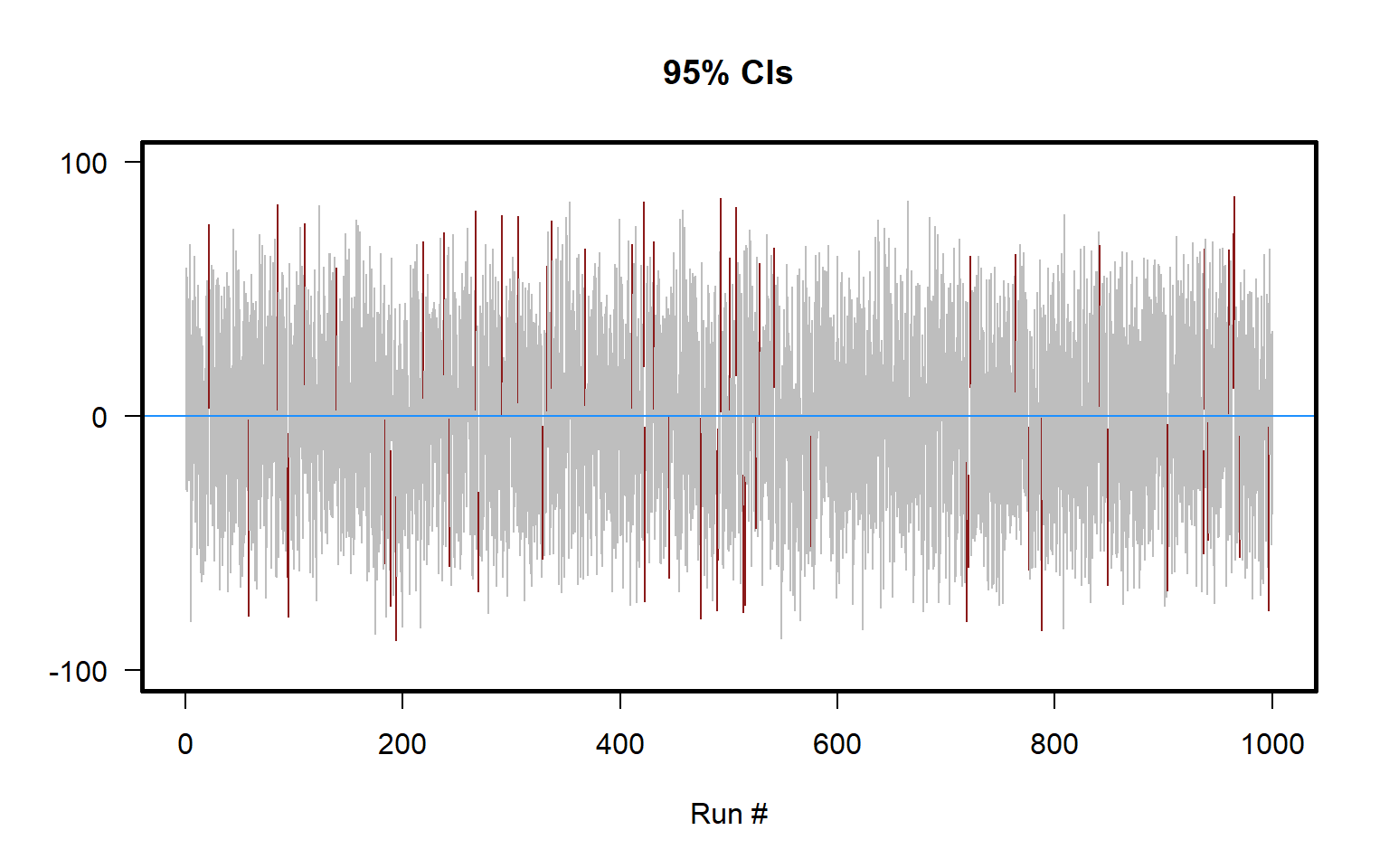
A 95% confidence interval can be conceptualized as a range of plausible values for an estimate. Remember that a population is the set of observations that we are interested in, and the sample is the set of observations that we have data for. A more precise conceptualization for a 95% confidence interval, is that, if we randomly sampled from a population over and over again, 95 percent of the 95% confidence intervals would contain the true population mean.

Let’s illustrate that with a simulation in the plot below, which plots 95% confidence intervals for samples of size n=10 drawn from a set of integers from -100 to +100. The 95% confidence intervals that contain the true population mean of zero are colored gray, and the 95% confidence intervals that do not contain the true population mean of zero are colored red. As illustrated in the plot, about 95 percent of the 95% confidence intervals contain the true population mean.

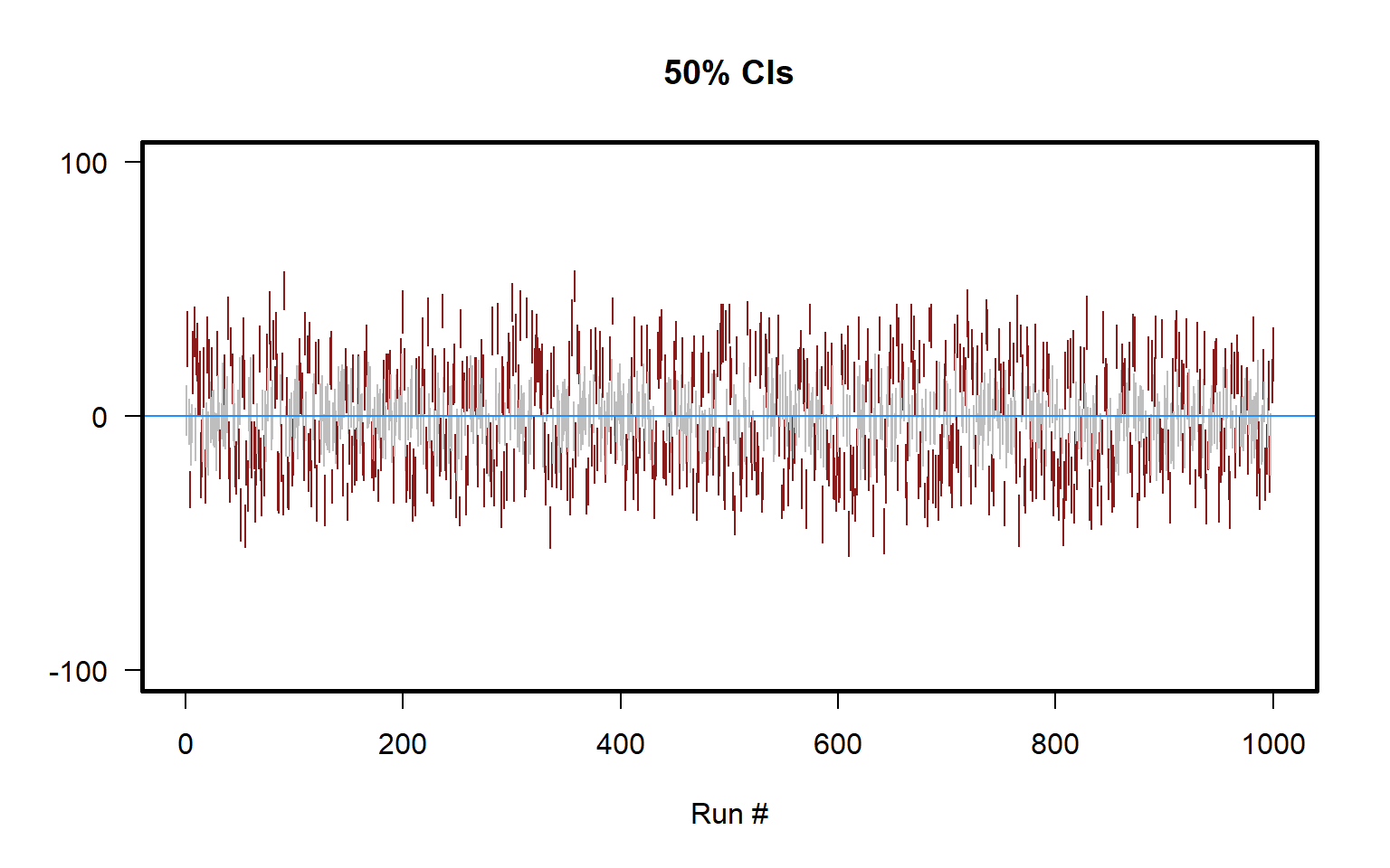
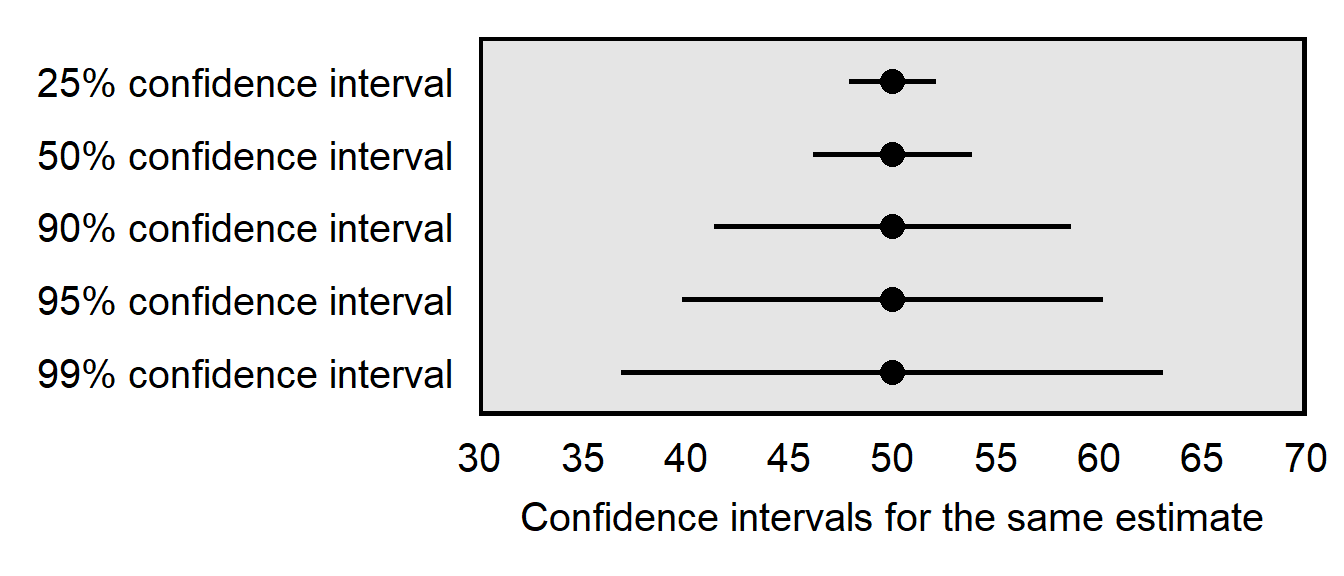
Sometimes percentages other than 95% are used to construct confidence intervals. The higher the percentage for a confidence interval, the wider the confidence interval must be to contain the true population mean. For example, a 99% confidence interval must contain the true mean 99 percent of the time, so a 99% confidence interval must be wider than a 95% confidence interval. And, the lower the percentage for a confidence interval, the thinner the confidence interval will be.

Below is a plot for 50% confidence intervals for the above situation of samples of size n=10 drawn from a set of numbers from -100 to +100. The plot indicates that only about 50 percent of the 50% confidence intervals contain the true mean (only about half of the lines are gray), and the plot also indicates that the 50% confidence intervals are not as wide as the 95% confidence intervals are for the same estimate.

Below is a plot of different confidence intervals for 50 heads in 100 flips of a coin, illustrating how having a higher confidence level requires a wider range of estimates.

So one factor that influences the width of a confidence interval is the associated percentage, such whether the confidence interval is a 95% confidence interval or a 50% confidence interval. Another factor that influences the width of a confidence interval is the sample size of the data that are used to construct the confidence interval: all else equal, larger random samples produce thinner confidence intervals, because the larger amount of data helps us “close in” on the true characteristics of the population.

The plot below illustrates how larger samples produce thinner confidence intervals, all else equal. For the plot, the underlying data are flips of a fair coin. The top row is for 10 flips that produced 5 heads and 5 tails, the second row is for 20 flips that produced 10 heads and 10 tails, and so forth.

SAMPLE SIZE	95% CONFIDENCE INTERVAL
10 flips	[19%, 81%]
20 flips	[28%, 72%]
100 flips	[40%, 60%]
200 flips	[43%, 57%]
1,000 flips	[47%, 53%]

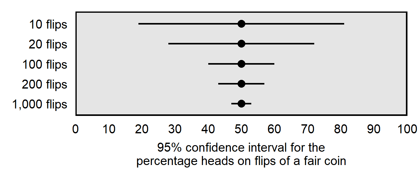
Notice that, in terms of reducing the width of the 95% confidence interval, adding 10 flips to 10 flips was more useful than adding 100 flips to 100 flips. This reflects the fact that, as sample size increases, a extra observation is not as useful as the prior observation has been.

Sample practice items

For a given estimate, all else equal, which one of the following would be the widest?

90% confidence interval
95% confidence interval
99% confidence interval

Answer

99% confidence interval

Suppose that we ask 1,000 U.S. residents to rate their support for the U.S. president on a scale from 0 to 100. The 95% confidence interval for the mean support for the president for the full sample is [40, 50]. The 99% confidence interval for the estimate for the full sample will be:

thinner than 10 units wide
wider than 10 units wide
10 units wide
there is not enough information to expect that any of these options is likely to occur

Answer

wider than 10 units wide
We need a wider range of values to be able to claim that the true value will be in the confidence interval 99% of the time.

Amy randomly samples 30 ISU students and asks them to rate the president on a scale from 0 for very cold to 100 for very warm. Bob randomly samples 200 ISU students and asks them to rate the president on a scale from 0 for very cold to 100 for very warm. Which of the following, if any, should be expected due to this difference in sample size?

The mean support for the president is lower in Amy’s sample than in Bob’s sample.
The mean support for the president is higher in Amy’s sample than in Bob’s sample.
Neither of the above

Answer

Neither of the above

The 95% confidence interval for mean support for the president is thinner in Amy’s sample than in Bob’s sample.
The 95% confidence interval for mean support for the president is thinner in Bob’s sample than in Amy’s sample.
Neither of the above

Answer

Bob has more data than Amy has, all else equal, so:
(B) The 95% confidence interval for mean support for the president is thinner in Bob’s sample than in Amy’s sample.

Suppose that we ask 1,000 U.S. residents to rate their support for the U.S. president on a scale from 0 to 100. The 95% confidence interval for the mean support for the president for the full sample is [40, 50]. Suppose that we lose a random half of these responses and re-calculate the 95% confidence interval for the remaining responses. That new 95% confidence interval will likely be:

thinner than 10 units wide
wider than 10 units wide
10 units wide
there is not enough information to expect that any of these options is likely to occur

Answer

wider than 10 units wide
We have less evidence, now that we lost data randomly.

2.8 Margin of error

Major learning objective(s) for this section:

Given a formula, calculate a margin of error.

Surveys sometimes report an estimate plus or minus a particular number, such as 50% \(\pm\) 3%. If the confidence interval isn’t explicitly indicated for an estimate, a plausible assumption is that the calculation was based on a 95% confidence interval, so 50% \(\pm\) 3% would indicate a 95% confidence interval of [47%, 53%].

Below is a formula that can be used to estimate a margin of error for a mean measured from a large random sample, using a 95% confidence interval, in which s is the sample standard deviation and n is the sample size. Standard deviation is in the numerator, so, all else equal, a larger standard deviation produces a larger margin of error. Sample size is in the denominator, so, all else equal, a larger sample size produces a smaller margin of error.

\[ MOE = 1.96 \times \frac{s}{\sqrt{n}} \] Below is a formula that can be used to calculate a margin of error for a proportion measured from a large random sample, using a 95% confidence interval, in which p is the sample proportion and n is the sample size:

\[ MOE = 1.96 \times \sqrt{\frac{(p)(1-p)}{n}} \] For a formula that uses percentages (from 0 to 100) for p instead of proportions (from 0 to 1):

\[ MOE = 1.96 \times \sqrt{\frac{(p)(100-p)}{n}} \]

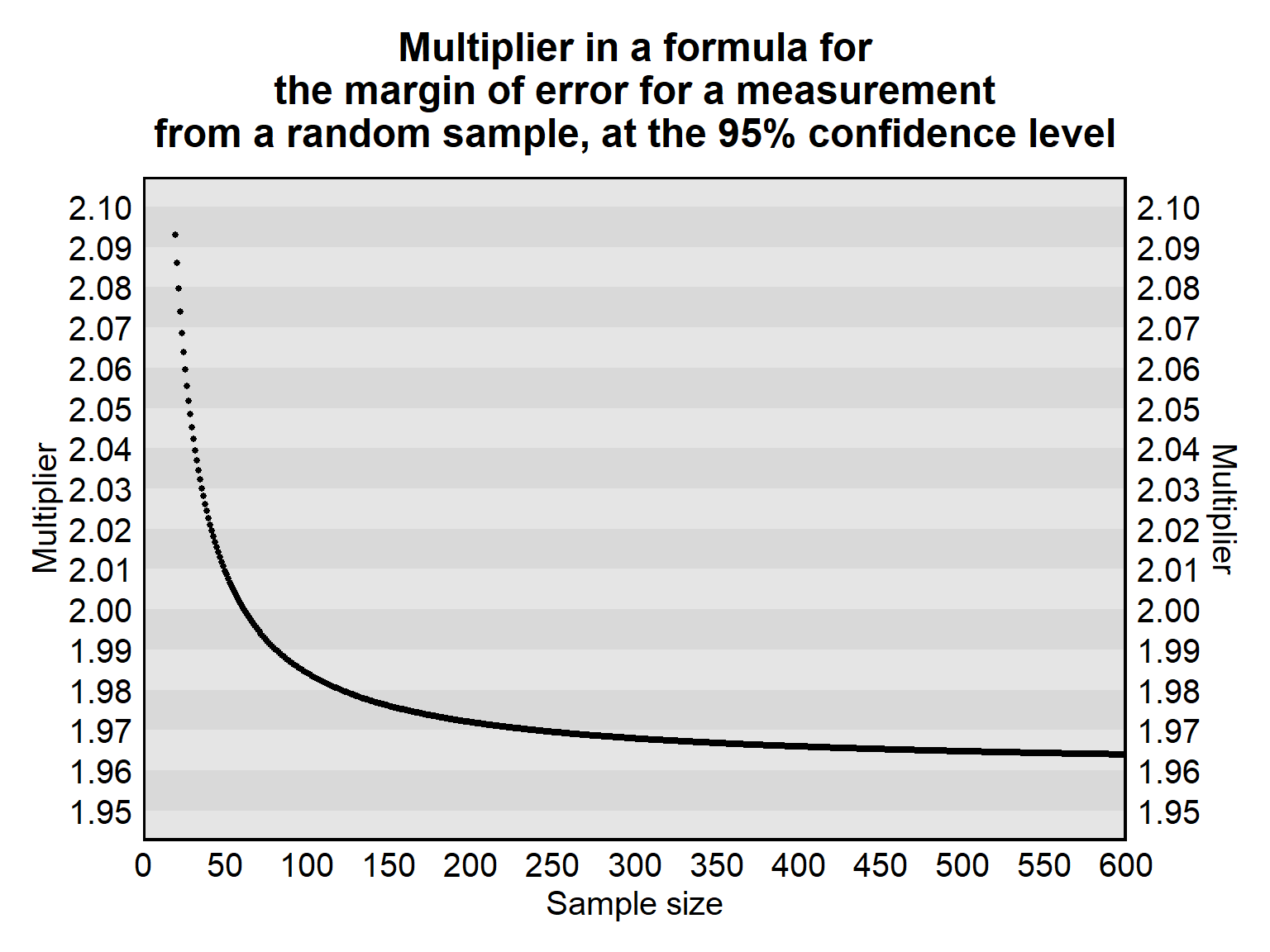
The front number 1.96 in the above formulas is the multiplier for a margin of error for a 95% confidence interval for a large sample. The multiplier that is used in a formula depends on the confidence interval percentage and the sample size. For example, the formula for the margin of error for a mean measured from a large random sample using a 99% confidence interval is:

\[ MOE = 2.58 \times \frac{s}{\sqrt{n}} \] If the margin of error is for a 95% confidence interval but the sample size is only 10, then the formula is:

\[ MOE = 2.26 \times \frac{s}{\sqrt{n}} \]

Tables are available online and elsewhere to determine the correct multiplier for a margin of error formula, but, for this POL 138 course, you will be given or referred to the appropriate formula. As indicated in the plot below, for a margin of error at the 95% confidence level, the multiplier is close to 1.96 for relatively large samples.

Such formulas used to calculate a margin of error are for random samples in which the only source of error is random sampling error. But sometimes some researchers use these formulas for samples that are not random. Using one of these margin of error formulas if the sample is not random can plausibly produce underestimates of the margin of error for an estimate, because a non-random sample plausibly has more sampling error than a random sample has.

Sample practice items

Suppose that, in a random sample of 256 Illinois residents, the mean rating about the governor on a scale from 0 to 100 was 68, and the standard deviation of the ratings was 24. Use the margin of error formula below to calculate the margin of error for the mean rating of the governor, in which s is the sample standard deviation and n is the sample size.

\[ MOE = 1.960 \times \frac{s}{\sqrt{n}} \]

Answer

\[ MOE = 1.960 \times \frac{24}{\sqrt{256}} = 2.94 \] So the margin of error for the mean rating is 2.94. So the estimated mean rating in the population is 68 \(\pm\) 3, if rounding to the nearest whole number.

Use the margin of error formula below to calculate the margin of error for an estimated percentage of persons who approve of the governor in a population, based on a random sample of the population in which 300 of 500 residents approved of the governor, in which p is the sample percentage and n is the sample size:

\[ MOE = 1.960 \times \sqrt{\frac{(p)(100-p)}{n}} \]

Answer

\[ MOE = 1.960 \times \sqrt{\frac{(60)(100-60)}{500}} = 2.19 \] So the margin of error for the percentage is 2.19%. So the estimated percentage of the population that approves of the governor is 60% \(\pm\) 2%, if rounding to the nearest whole number.