4 Linear regression
4.1 Simple linear regression
Major learning objective(s) for this section:
- Interpret an X/Y plot.
- Interpret coefficients and p-values from a simple linear regression.
A simple linear regression involves two variables. For a simple linear regression, a straight line of best fit is drawn through the center of the set of observations, to indicate the general association between the two variables. The plot below illustrates this, using variation in an X variable on the horizontal axis (the number of police officers per 100,000 residents in a state in the United States in 2018), to predict variation in a Y variable on the vertical axis (the number of homicides per 100,000 residents in the state in 2018). Each point in the plot represents one of the 50 states in the United States.
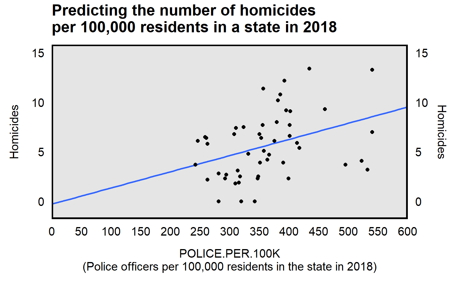
Statistical software can draw the straight line of best fit through the points and can report statistical output about this line of best fit, like below:
## MODEL INFO:
## Observations: 50
## Dependent Variable: HOMICIDES.PER.100K
## Type: OLS linear regression
##
## Standard errors:OLS
## ----------------------------------------------------------------
##                           Est.     2.5%   97.5%   t val.       p
## --------------------- -------- -------- ------- -------- -------
## (Intercept)             -0.290   -4.701   4.121   -0.132   0.895
## POLICE.PER.100K          0.016    0.004   0.028    2.748   0.008
## ----------------------------------------------------------------
The linear regression output has a few important numbers. Let’s start with the -0.290 estimate for the intercept. The intercept for a linear regression is the predicted outcome when all predictors are set to zero. In this case, the intercept indicates that the predicted homicide rate per 100,000 residents is -0.290 for a state that had zero police officers. It’s impossible to have a negative homicide rate, but linear regression merely draws a line of best fit through points, and there is nothing to stop the linear regression from producing predictions that are impossible.
For our analysis, a more important number is the 0.016 estimate on the POLICE.PER.100K predictor. For a linear regression, the estimate for a predictor can be thought of as a slope: for a one-unit increase in the predictor, the predicted outcome changes by the coefficient for the predictor. In this case, the 0.016 coefficient estimate indicates that, for each one-unit increase in POLICE.PER.100K, the HOMICIDES.PER.100K outcome is predicted to increase by 0.016. That positive coefficient indicates that states with a higher number of police officers per 100,000 residents are predicted to have a higher homicide rate, on average, compared to states with a lower number of police officers per 100,000 residents.
Notice that the linear regression coefficient estimates can be placed in the formula for a line: Y = mX + b, in which m is the slope and b is the y-intercept:
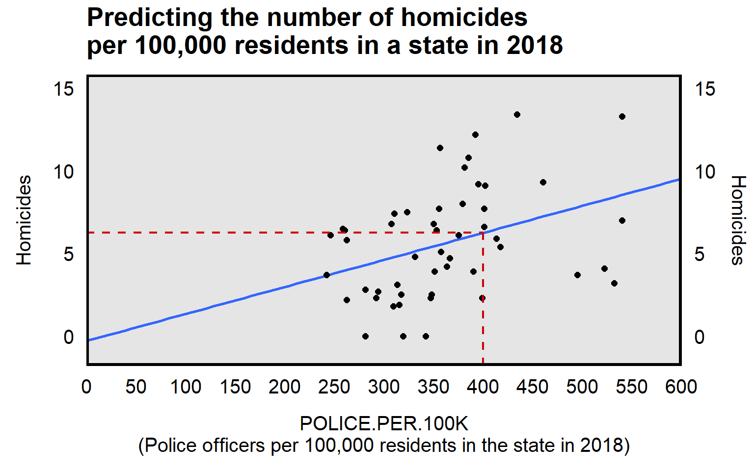
HOMICIDES.PER.100K = 0.016*POLICE.PER.100K + -0.290We can use this formula to make predictions. Let’s calculate the predicted number of homicides per 100,000 residents for a state that had 400 police officers per 100,000 residents:
HOMICIDES.PER.100K = 0.016*POLICE.PER.100K + -0.290
HOMICIDES.PER.100K = 0.016*400             + -0.290
HOMICIDES.PER.100K = 6.11
That prediction merely tells us where the X and Y meet the line of best fit, as indicated by the red dashed line:
Often a linear regression equation places the intercept first:
HOMICIDES.PER.100K = -0.290 + 0.016*POLICE.PER.100K
But the order of the terms of the equation doesn’t change the predictions.
Note on terminology
The R output indicates the “dependent” variable. This is a term that refers to the outcome variable that we are trying to predict.
Sample practice items
The output below is based on survey data from the ANES 2016 Time Series Study. The output is for an analysis that uses respondent years of age (a variable called “AGE”, coded from 18 to 90) to predict respondent feeling thermometer ratings about police (a variable called “FTPOLICE”, coded from 0 for very cold ratings to 100 for very warm ratings):
## MODEL INFO:
## Observations: 3538 (732 missing obs. deleted)
## Dependent Variable: FTPOLICE
## Type: OLS linear regression
##
## Standard errors:OLS
## ---------------------------------------------------------
##                      Est.    2.5%   97.5%   t val.      p
## ----------------- ------- ------- ------- -------- ------
## (Intercept)         62.27   60.10   64.43    56.34   0.00
## AGE                  0.27    0.23    0.31    12.66   0.00
## ---------------------------------------------------------
The intercept coefficient of 62.27 indicates the predicted rating about police among…
- respondents who are zero years old
- respondents who are 18 years old
- respondents who are the average age among respondents
- respondents who are 62.27 years old
Answer
- respondents who are zero years old
What does the age coefficient of 0.27 indicate?
- How much the predicted rating about police changes for each one-unit increase in age
- The difference in predicted ratings about police between a young respondent and an old respondent
- The predicted rating about police among a respondent zero years old
- The predicted rating about police among a respondent at the average age among respondents
Answer
- How much the predicted rating about police changes for each one-unit increase in age
Based on the linear regression output, what would be the predicted rating about police from a 50-year-old respondent, to two decimal places?
- 13.5
- 48.9
- 62.3
- 75.8
Answer
- 75.8
62.27 + 0.27*50 = 75.8
Let’s use the linear regression below, which uses a measure of respondent age to predict respondent ratings about the U.S. Congress (FTCONGRESS), based on data from the ANES 2016 Time Series Study:
## MODEL INFO:
## Observations: 3523 (747 missing obs. deleted)
## Dependent Variable: FTCONGRESS
## Type: OLS linear regression
##
## Standard errors:OLS
## -------------------------------------------------------------
##                       Est.     2.5%    97.5%   t val.       p
## ----------------- -------- -------- -------- -------- -------
## (Intercept)         45.887   43.690   48.084   40.948   0.000
## AGE                 -0.064   -0.105   -0.022   -2.977   0.003
## -------------------------------------------------------------
What does the 45.887 coefficient for the intercept indicate?
- The predicted mean rating about the U.S. Congress is 45.887.
- The predicted mean rating about the U.S. Congress is 45.887 among respondents who are 18 years old.
- The predicted mean rating about the U.S. Congress is 45.887 among respondents who are 0 years old.
Answer
- The predicted mean rating about the U.S. Congress is 45.887 among respondents who are 0 years old.
What does the -0.064 coefficient estimate for age indicate?
- The mean rating about the U.S. Congress is -0.064.
- The predicted mean rating about the U.S. Congress changes by -0.064 for each one-unit increase in age.
- The predicted mean rating about the U.S. Congress is 0.064 lower for old respondents than for young respondents.
Answer
- The predicted mean rating about the U.S. Congress changes by -0.064 for each one-unit increase in age.
Does the analysis provide sufficient evidence at the conventional level in political science that, at least in these data, respondent age associates with respondent ratings about the U.S. Congress?
- Yes
- No
Answer
- Yes
Does the analysis provide sufficient evidence at the conventional level in political science that, at least in these data and at least on average, respondents getting older caused respondent ratings about the U.S. Congress to get lower?
- Yes
- No
Answer
- No
Let’s practice interpreting a linear regression, using survey data from the ANES 2016 Time Series Study. The output below predicts a participant’s ratings about Donald Trump (FTTRUMP) using a predictor for the participant’s age in years (AGE):
## MODEL INFO:
## Observations: 3536 (734 missing obs. deleted)
## Dependent Variable: FTTRUMP
## Type: OLS linear regression
##
## Standard errors:OLS
## ---------------------------------------------------------
##                      Est.    2.5%   97.5%   t val.      p
## ----------------- ------- ------- ------- -------- ------
## (Intercept)         30.04   26.62   33.45    17.24   0.00
## AGE                  0.24    0.18    0.31     7.31   0.00
## ---------------------------------------------------------
What does the 30.04 coefficient estimate for the intercept indicate?
- The mean rating about Donald Trump is predicted to be 30.04.
- The mean rating about Donald Trump is predicted to be 30.04 among participants of age zero.
- The mean rating about Donald Trump is predicted to be 30.04 among participants of the average age.
- The mean rating about Donald Trump is predicted to increase 30.04 for a one-unit increase in participant age.
- The mean rating about Donald Trump is predicted to be 30.04 units higher for old participants than for young participants.
Answer
- The mean rating about Donald Trump is predicted to be 30.04 among participants of age zero.
What does the 0.24 coefficient estimate for AGE indicate?
- The mean rating about Donald Trump is predicted to be 0.24.
- The mean rating about Donald Trump is predicted to be 0.24 among participants of age zero.
- The mean rating about Donald Trump is predicted to be 0.24 among participants of the average age.
- The mean rating about Donald Trump is predicted to increase 0.24 for a one-unit increase in participant age.
- The mean rating about Donald Trump is predicted to be 0.24 units higher for old participants than for young participants.
Answer
- The mean rating about Donald Trump is predicted to increase 0.24 for a one-unit increase in participant age.
Of the following, which are justified interpretations of the p-value p<0.05 for the 0.24 coefficient estimate for AGE?
- The p-value indicates that there is sufficient evidence at the conventional level in political science that participant age positively associates with ratings about Donald Trump, at least among these participants and at least on average.
- The p-value indicates that there is sufficient evidence at the conventional level in political science that getting older causes a participant to have higher ratings about Donald Trump, at least among these participants and at least on average.
- Both of the above
- Neither of the above
Answer
- The p-value indicates that there is sufficient evidence at the conventional level in political science that participant age positively associates with ratings about Donald Trump, at least among these participants and at least on average.
4.2 Drawing the line of best fit
Major learning objective(s) for this section:
- Use linear regression output to draw a regression line on an X/Y plot.
Let’s use the linear regression below, which uses a measure of respondent partisanship (PARTY06, which is coded from 0 for Strong Democrat to 6 for Strong Republican) to predict respondent ratings about feminists (FTFEMINISTS), based on data from the ANES 2016 Time Series Study:
## MODEL INFO:
## Observations: 3564 (706 missing obs. deleted)
## Dependent Variable: FTFEMINISTS
## Type: OLS linear regression
##
## Standard errors:OLS
## ---------------------------------------------------------
## Est. 2.5% 97.5% t val. p
## ----------------- ------- ------- ------- -------- ------
## (Intercept) 71.20 69.92 72.47 109.44 0.00
## PARTY06 -5.32 -5.68 -4.96 -29.17 0.00
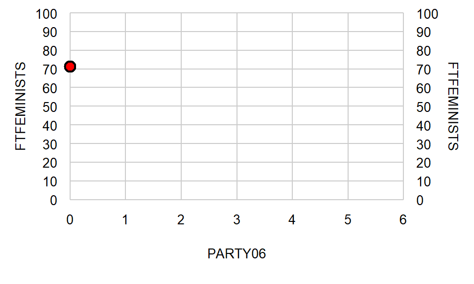
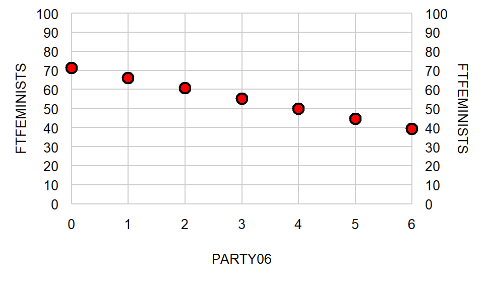
## ---------------------------------------------------------Let’s plot the linear regression line on an X/Y axis. Let’s start by plotting the y-intercept of 71.20:
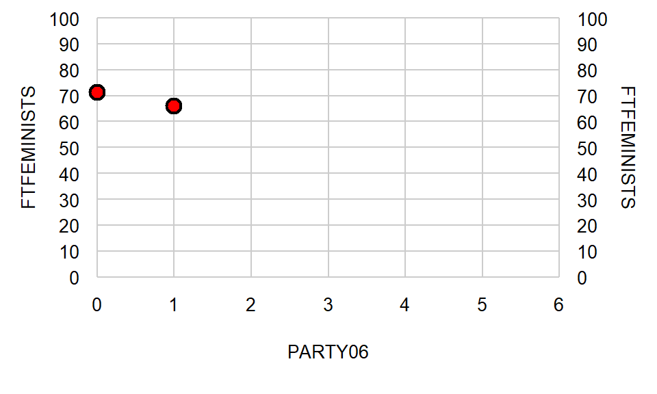
Now let’s calculate the predicted outcome after a one-unit increase in the predictor, so for when PARTY06 is 1:
Y = 71.20 + (-5.32 * PARTY06)
Y = 71.20 + (-5.32 * 1)
Y = 71.20 + (-5.32)
Y = 65.88
Let’s get predictors for additional one-unit increases in PARTY06, in which each one-unit increase in PARTY06 associates with a decrease of 5.32 in the FTFEMINISTS outcome:
Now let’s draw a line through our points:
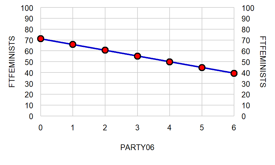
For drawing a line of best fit from statistical output, a shortcut is to plot the leftmost point for X (in this case, at PARTY06 of 0), plot the rightmost point for X (in this case, at PARTY06 of 6), and draw a line between those two points.
Sample practice items
Below are coefficient estimates from a linear regression of data from residents in a hypothetical country. The linear regression used the number of years of education of a resident (X) to predict the resident’s support for the country’s president (Y).
Coefficients:
                    Estimate
(Intercept)      70.00
Education        -3.00
- Write the equation to predict Y using X.
- Label the Y-axis and the X-axis on the graph.
- Draw and label a point at the value of Y for which the X variable is 10 (the lowest observed level of education).
- Draw and label a point at the value of Y for which the X variable is 20 (the highest observed level of education).
- Draw a line between the above two points.
Answer
[1] Y = 70 + -3X[3] Plug in X=10 to get: Y=70+-310 = 70-30=40. Plot a point at X=10, Y=40
[4] Plug in X=20 to get: Y=70+-320 = 70-60=10. Plot a point at X=10, Y=10
4.3 Linear regression with categorical predictors
Major learning objective(s) for this section:
- Interpret coefficients and p-values from a linear regression that has a categorical predictor.
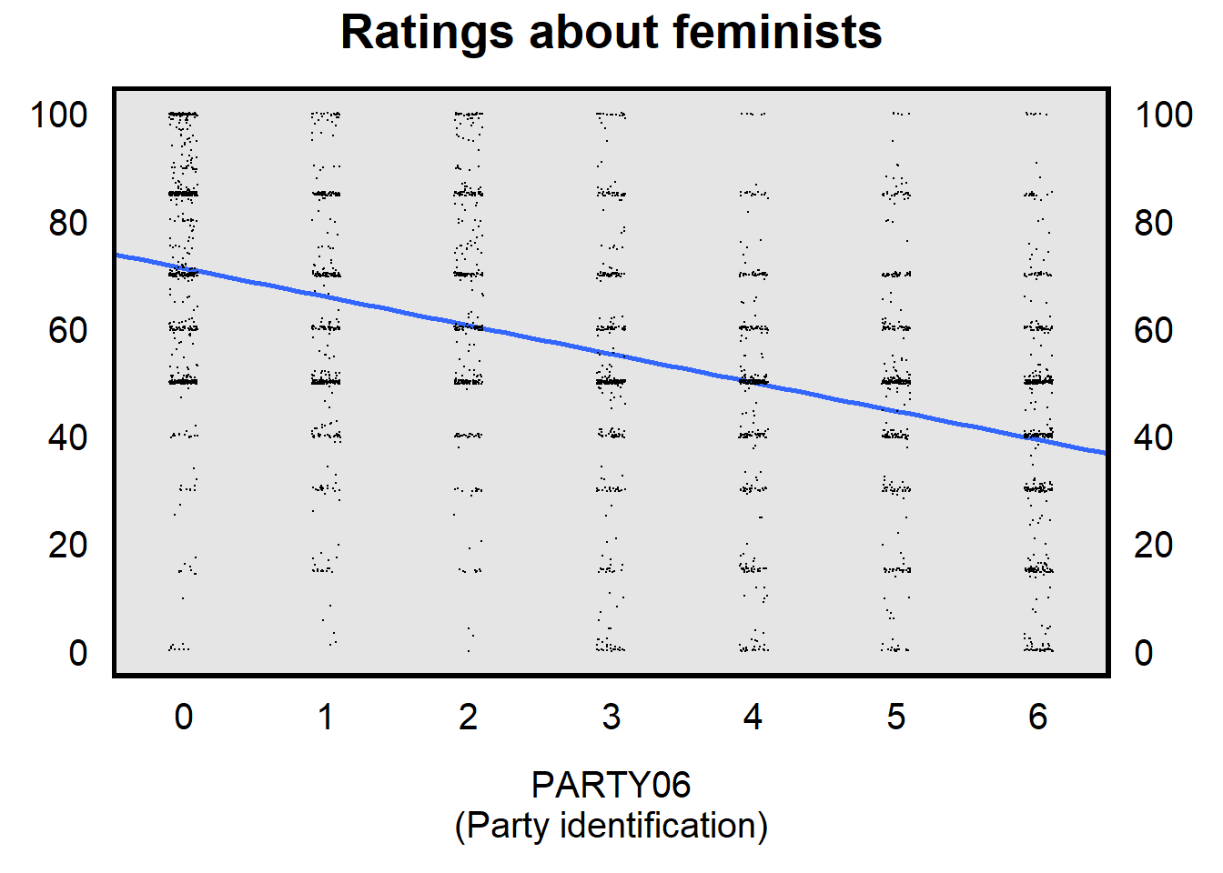
Let’s use survey data from the ANES 2016 Time Series Study to illustrate how to read statistical output for categorical predictors in a linear regression. Like above, the outcome variable is respondent feeling thermometer ratings about feminists (a variable called “FTFEMINISTS”, coded from 0 to 100). Our predictor is PARTY06, which is participant partisan identification, on a scale that has seven levels that range from 0 for “strong Democrat” to 6 for “strong Republican”. The plot below has dots to indicate the observations (jittered a bit left or right, so that we can see more of the observations that would otherwise be on top of each other). The blue line in the plot below is the line of best fit through these points, which indicates an on-average negative association between PARTY06 and FTFEMINISTS.
Below is the statistical output for this blue regression line. The 71.20 coefficient for the intercept indicates the y-intercept of the line. This y-intercept indicates the predicted value of the outcome when all predictors are set to zero. In this case, when PARTY06 is zero, that’s a strong Democrat, so the mean predicted value of FTFEMINISTS is 71.20 among strong Democrats. The -5.32 coefficient for PARTY06 indicates the slope of the line. The slope of the line indicates the change in the predicted outcome for a one-unit change in the predictor. In this case, as PARTY06 changes from, say, 0 to 1, the predicted value of FTFEMINISTS changes from 71.20 to (71.20 + -5.32), so that the mean predicted value of FTFEMINISTS is 65.88 among not strong Democrats.
## MODEL INFO:
## Observations: 3564 (706 missing obs. deleted)
## Dependent Variable: FTFEMINISTS
## Type: OLS linear regression
##
## Standard errors:OLS
## ---------------------------------------------------------
##                      Est.    2.5%   97.5%   t val.      p
## ----------------- ------- ------- ------- -------- ------
## (Intercept)         71.20   69.92   72.47   109.44   0.00
## PARTY06             -5.32   -5.68   -4.96   -29.17   0.00
## ---------------------------------------------------------
The y-intercept and slope of the line can be used to write a formula for calculating predicted values of the outcome, using the format Y=mX + b. In this case, and placing b before mX:
FTEMINISTS = 71.20 + (-5.32 * PARTY06)
So the predicted value of FTFEMINISTS among strong Republicans would be:
FTEMINISTS = 71.20 + (-5.32 * PARTY06)
FTEMINISTS = 71.20 + (-5.32 * 6)
FTEMINISTS = 71.20 + (-31.92)
FTEMINISTS = 39.28
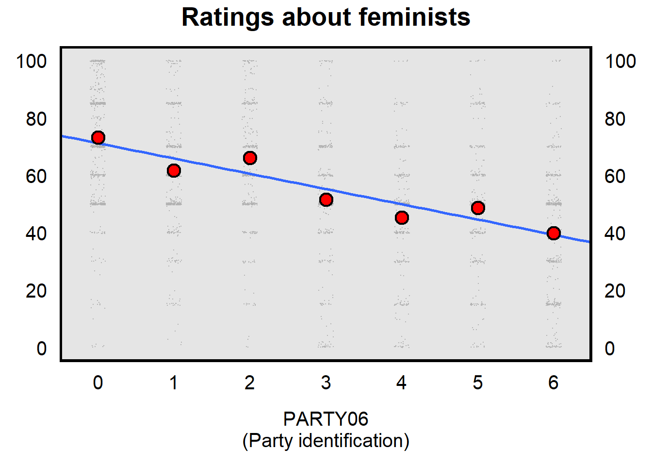
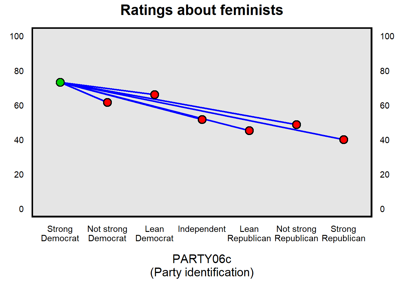
Our original linear regression using PARTY06 to predict FTFEMINISTS used a single line of best fit. That line of best fit makes better predictions than random guessing, but a single line of best fit isn’t the best that we can do. Check the plot below, in which the red dots indicate the mean value of FTFEMINISTS at different levels of PARTY06. The line of best fit prediction is close for PARTY06 of 0 and PARTY06 of 6, but is too high for PARTY06 of 2 and is too low for PARTY06 of 3.
To improve our predictions, we can code PARTY06 as a categorical predictor (PARTYc) and then make separate predictions for each category of PARTY06c. Let’s conduct a linear regression doing that, below:
Below is the linear regression output:
## MODEL INFO:
## Observations: 3564 (706 missing obs. deleted)
## Dependent Variable: FTFEMINISTS
## Type: OLS linear regression
##
## Standard errors:OLS
## --------------------------------------------------------------------------
##                                     Est.     2.5%    97.5%   t val.      p
## ------------------------------- -------- -------- -------- -------- ------
## (Intercept)                        73.08    71.43    74.74    86.57   0.00
## PARTY06cNot strong                -11.50   -14.17    -8.84    -8.46   0.00
## Democrat
## PARTY06cLean Democrat              -7.07    -9.83    -4.31    -5.02   0.00
## PARTY06cIndependent               -21.51   -24.19   -18.84   -15.78   0.00
## PARTY06cLean Republican           -27.89   -30.62   -25.17   -20.06   0.00
## PARTY06cNot strong                -24.47   -27.21   -21.73   -17.53   0.00
## Republican
## PARTY06cStrong Republican         -33.18   -35.67   -30.69   -26.09   0.00
## --------------------------------------------------------------------------
For the categorical predictor above – and for all categorical predictors – one of the categories much be omitted, to be used as the reference category. This reference category is placed into the intercept. In the linear regression above, the omitted category is “Strong Democrat”, and all other categories are interpreted relative to the omitted category. So the intercept of 73.08 is the predicted level of FTFEMINISTS among the omitted category of strong Democrat. The -11.50 coefficient for not strong Democrat indicates that the predicted level of FTFEMINISTS among not strong Democrats is 11.50 units below the predicted level of FTFEMINISTS among the omitted category of strong Democrat (so that’s 73.08 minus 11.50, which is 61.58). The -7.07 coefficient for Lean Democrat indicates that the predicted level of FTFEMINISTS among participants who lean Democrat is 7.07 units below the predicted level of FTFEMINISTS among the omitted category of strong Democrat (so that’s 73.08 minus 7.07, which is 66.01).
Just like before, we can write an equation for the predictions:
FTEMINISTS = 73.08
             + -11.50*(Not strong Democrat)
             +  -7.07*(Lean Democrat)
             + -21.51*(Independent)
             + -27.89*(Lean Republican)
             + -24.47*(Not strong Republican)
             + -33.18*(Strong Republican)
Important note: For a categorical predictor, the coefficient always refers to a comparison with the omitted category. The numeric coding of a predictor does not matter when the predictor is used in a regression as a categorical predictor. The PARTY06c variable is coded so that Strong Republican is coded 6, but the calculation of the coefficient for the “Strong Republican” category of PARTY06c does not use this 6. So, for example, to get the predicted level of FTFEMINISTS among Strong Republicans, we start with the intercept of 73.08 and then add in the -33.18 coefficient for Strong Republican, to get a predicted FTFEMINISTS level of 39.90 among Strong Republicans. For a categorical predictor, do not multiply the -33.18 coefficient for Strong Republican by the numeric coding of 6 for Strong Republican. The -33.18 is essentially multiplied only by 1, because the -33.18 coefficient indicates the predicted change from the omitted category to the Strong Republican category.
Let’s illustrate that below, by plugging in 0 if the Strong Republican category is not used and 1 if the Strong Republican category is used.
FTEMINISTS = 73.08
             + -11.50*(Not strong Democrat)
             +  -7.07*(Lean Democrat)
             + -21.51*(Independent)
             + -27.89*(Lean Republican)
             + -24.47*(Not strong Republican)
             + -33.18*(Strong Republican)

FTEMINISTS = 73.08
             + -11.50*(0)
             +  -7.07*(0)
             + -21.51*(0)
             + -27.89*(0)
             + -24.47*(0)
             + -33.18*(1)

FTEMINISTS = 39.90
Let’s do another example, to get the predicted level of FTEMINISTS among a Lean Democrat respondent:
FTEMINISTS = 73.08
             + -11.50*(Not strong Democrat)
             +  -7.07*(Lean Democrat)
             + -21.51*(Independent)
             + -27.89*(Lean Republican)
             + -24.47*(Not strong Republican)
             + -33.18*(Strong Republican)

FTEMINISTS = 73.08
             + -11.50*(0)
             +  -7.07*(1)
             + -21.51*(0)
             + -27.89*(0)
             + -24.47*(0)
             + -33.18*(0)

FTEMINISTS = 66.01
Let’s conduct the same linear regression but exclude the “Independent” category:
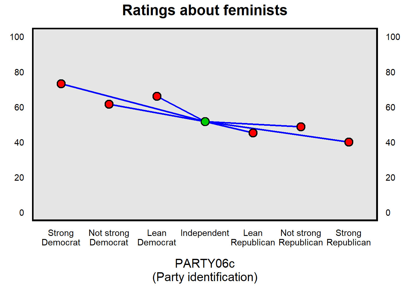
Below is the linear regression output, in which the intercept of 51.57 is now the predicted outcome among the omitted category, of Independents.
## MODEL INFO:
## Observations: 3564 (706 missing obs. deleted)
## Dependent Variable: FTFEMINISTS
## Type: OLS linear regression
##
## Standard errors:OLS
## -------------------------------------------------------------------------
##                                     Est.     2.5%   97.5%   t val.      p
## ------------------------------- -------- -------- ------- -------- ------
## (Intercept)                        51.57    49.47   53.67    48.18   0.00
## PARTY06cStrong Democrat            21.51    18.84   24.19    15.78   0.00
## PARTY06cNot strong                 10.01     7.05   12.97     6.63   0.00
## Democrat
## PARTY06cLean Democrat              14.45    11.40   17.49     9.29   0.00
## PARTY06cLean Republican            -6.38    -9.40   -3.36    -4.15   0.00
## PARTY06cNot strong                 -2.96    -5.98    0.07    -1.92   0.06
## Republican
## PARTY06cStrong Republican         -11.67   -14.47   -8.86    -8.15   0.00
## -------------------------------------------------------------------------
Just like before, we can write an equation for the predictions:
FTEMINISTS = 51.57
             +  21.51*(Strong Democrat)
             +  10.01*(Not strong Democrat)
             +  14.45*(Lean Democrat)
             +  -6.38*(Lean Republican)
             +  -2.96*(Not strong Republican)
             + -11.67*(Strong Republican)
So if we wanted to get a prediction for a participant who leans Democrat:
FTEMINISTS = 51.57
             +  21.51*(Strong Democrat)
             +  10.01*(Not strong Democrat)
             +  14.45*(Lean Democrat)
             +  -6.38*(Lean Republican)
             +  -2.96*(Not strong Republican)
             + -11.67*(Strong Republican)

FTEMINISTS = 51.57
             +  21.51*(0)
             +  10.01*(0)
             +  14.45*(1)
             +  -6.38*(0)
             +  -2.96*(0)
             + -11.67*(0)

FTEMINISTS = 51.57
             + 14.45

FTEMINISTS = 66.02
That 66.02 prediction for lean Democrat from the regression that omitted the Independent category is the same as the 66.01 prediction from the regression that omitted the strong Republican category, with the difference due only to rounding error.
Sample practice items
Let’s predict a participant’s ratings about Donald Trump, but let’s use a predictor for the participant’s race, coded as “White”, “Black”, “Asian”, or “Other race”, with “Other race” as the omitted category:
## MODEL INFO:
## Observations: 3632 (638 missing obs. deleted)
## Dependent Variable: FTTRUMP
## Type: OLS linear regression
##
## Standard errors:OLS
## -----------------------------------------------------------
##                       Est.     2.5%   97.5%   t val.      p
## ----------------- -------- -------- ------- -------- ------
## (Intercept)          32.38    29.58   35.19    22.63   0.00
## RACEWhite            14.75    11.66   17.84     9.36   0.00
## RACEBlack           -11.72   -16.29   -7.15    -5.03   0.00
## RACEAsian             5.09    -1.72   11.91     1.46   0.14
## -----------------------------------------------------------
What does the 32.38 coefficient estimate for the intercept indicate?
- The mean rating about Donald Trump is predicted to be 32.38.
- The mean rating about Donald Trump is predicted to be 32.38 among “Other race” participants.
- The mean rating about Donald Trump is predicted to increase by 32.38 for a one-unit increase in participant race.
- The mean rating about Donald Trump is predicted to be 32.38 units higher for “Other race” participants than for residual participants.
Answer
- The mean rating about Donald Trump is predicted to be 32.38 among “Other race” participants.
What does the 14.75 coefficient estimate for RACEWhite indicate?
- The mean rating about Donald Trump is predicted to be 14.75 among White participants.
- The mean rating about Donald Trump is predicted to be 14.75 higher among White participants than among all other participants.
- The mean rating about Donald Trump is predicted to be 14.75 higher among White participants than among “Other race” participants.
Answer
- The mean rating about Donald Trump is predicted to be 14.75 higher among White participants than among “Other race” participants.
Of the following, which are justified interpretations of the p-value p=0.14 for the coefficient estimate for RACEAsian?
- The p-value indicates that there is insufficient evidence at the conventional level in political science that Asians rate Donald Trump any different on average than all other participants rate Donald Trump.
- The p-value indicates that there is insufficient evidence at the conventional level in political science that Asians rate Donald Trump any different on average than “Other race” participants rate Donald Trump.
Answer
- The p-value indicates that there is insufficient evidence at the conventional level in political science that Asians rate Donald Trump any different on average than “Other race” participants rate Donald Trump.