14 Statistical tests in R
Microsoft Excel can be used for a lot of statistical calculations, but Microsoft Excel isn’t ideal for advanced statistical analysis, because, among other reasons, Excel is relatively difficult to check work for. For example, if I want to check whether you used the correct formulas, I would need to do something such as click in each cell that has a formula and check that formula. Other programs, though, permit readers to view the formulas directly.
One of the more advanced statistical programming language is R, which you can access in ISU campus computer labs, or by downloading R to your computer, or at websites such as WebR. Let’s practice statistical tests in R.
14.1 Binomial test
Major learning objective(s) for this section:
- Draft and execute an R command to test a null hypothesis, using a binomial test.
- Interpret the result from statistical tests in R.
The binomial test can be used to test the null hypothesis that an observed proportion equals a specific proportion. Let’s use R to test the null hypothesis that a coin is fair, based on our observations of the coin. For this, we can use a binomial test of the form…
binom.test(x, n, p)
…in which x is the number of successes, n is the number of observations, and the p is the probability of success for each observation. In our case, we can define success as getting heads on each flip, so that the probability p is 0.50.
Let’s run the binomial test to test the null hypothesis that a coin is fair, based on observations of a coin that landed on heads 5 times in 10 flips:
##
##  Exact binomial test
##
## data:  5 and 10
## number of successes = 5, number of trials = 10, p-value = 1
## alternative hypothesis: true probability of success is not equal to 0.5
## 95 percent confidence interval:
##  0.187086 0.812914
## sample estimates:
## probability of success
##                    0.5
In this case, the p-value is 1, because 5 heads and 5 tails provides no evidence against the null hypothesis that the coin is fair.
Let’s run the binomial test to test the null hypothesis that a coin is fair, based on observations of a coin that landed on heads 4 times in 10 flips:
##
##  Exact binomial test
##
## data:  4 and 10
## number of successes = 4, number of trials = 10, p-value = 0.7539
## alternative hypothesis: true probability of success is not equal to 0.5
## 95 percent confidence interval:
##  0.1215523 0.7376219
## sample estimates:
## probability of success
##                    0.4
In this case, the p-value is less than 1, because the 4 heads and 6 tails provides some evidence against the null hypothesis that the coin is fair.
Let’s run the binomial test to test the null hypothesis that a coin is fair, based on observations of a coin that landed on heads 0 times in 10 flips:
##
##  Exact binomial test
##
## data:  0 and 10
## number of successes = 0, number of trials = 10, p-value = 0.001953
## alternative hypothesis: true probability of success is not equal to 0.5
## 95 percent confidence interval:
##  0.0000000 0.3084971
## sample estimates:
## probability of success
##                      0
In this case, the p-value is less than 1, because 0 heads and 10 tails provides some evidence against the null hypothesis that the coin is fair. Moreover, the p-value is even lower than the p-value for 4 heads in 10 flips, because 0 heads in 10 flips provides even more evidence against the null hypothesis that the coin is fair, compared to the evidence provided by 4 heads in 10 flips.
R will sometimes report small p-values using scientific notation. For example, below is output for a test of the null hypothesis that a coin is fair, based on a coin that landed on heads 0 times in 20 flips:
##
##  Exact binomial test
##
## data:  0 and 20
## number of successes = 0, number of trials = 20, p-value = 1.907e-06
## alternative hypothesis: true probability of success is not equal to 0.5
## 95 percent confidence interval:
##  0.0000000 0.1684335
## sample estimates:
## probability of success
##                      0
The p-value of “1.907e-06” is written in scientific notation and indicates 1.907 \(\times\) 10-6. An easy way to remember how to interpret scientific notation is that the exponent indicates how many places to move the decimal point, and the sign on the exponent indicates the direction to move the decimal point, with a positive number indicating to move the decimal point right (to make the number larger) and a negative number indicating to move the decimal point to the left (to make the number smaller). So 1.907 \(\times\) 10-6 can be thought of as 0000001.907 \(\times\) 10-6, so that moving the decimal point six places to the left will produce 0.000001907.
Scientific notation in R can be shut off with the command “options(scipen=999)”:
##
##  Exact binomial test
##
## data:  0 and 20
## number of successes = 0, number of trials = 20, p-value = 0.000001907
## alternative hypothesis: true probability of success is not equal to 0.5
## 95 percent confidence interval:
##  0.0000000 0.1684335
## sample estimates:
## probability of success
##                      0
The binom.test command does not require equal sign assignments, such as “x = 0”. If equal sign assignments are omitted from the binom.test command, R will assume that the first number is x, the second number is n, and the third number is p.
Compare the output for this binom.test command that has equal sign assignments…
##
##  Exact binomial test
##
## data:  0 and 20
## number of successes = 0, number of trials = 20, p-value = 0.000001907
## alternative hypothesis: true probability of success is not equal to 0.5
## 95 percent confidence interval:
##  0.0000000 0.1684335
## sample estimates:
## probability of success
##                      0
…to this binom.test command that does not have equal sign assignments:
##
##  Exact binomial test
##
## data:  0 and 20
## number of successes = 0, number of trials = 20, p-value = 0.000001907
## alternative hypothesis: true probability of success is not equal to 0.5
## 95 percent confidence interval:
##  0.0000000 0.1684335
## sample estimates:
## probability of success
##                      0
Equal sign assignments can be useful to override the default order of x/n/pr:
##
##  Exact binomial test
##
## data:  0 and 20
## number of successes = 0, number of trials = 20, p-value = 0.000001907
## alternative hypothesis: true probability of success is not equal to 0.5
## 95 percent confidence interval:
##  0.0000000 0.1684335
## sample estimates:
## probability of success
##                      0
Sample practice items
Which of the following is an R command that uses a binomial test to test the null hypothesis that a coin is fair, for a coin that lands on heads 3 times and lands on tails 1 time in 4 flips?
- binom.test(x = 3, n = 4, p = 0.5)
- binom.test(x = 4, n = 3, p = 0.5)
- binom.test(x = 3, n = 1, p = 0.5)
- binom.test(x = 1, n = 3, p = 0.5)
- None of the above
Answer
- binom.test(x = 3, n = 4, p = 0.5)
14.2 Fisher’s exact test
Major learning objective(s) for this section:
- Draft and execute an R command to test a null hypothesis, using a Fisher’s exact test.
- Interpret the result from statistical tests in R.
Fisher’s exact test can be used to test the null hypothesis that a proportion in one sample equals a proportion in another sample. Imagine a hypothetical randomized experiment that has a control group of 100 participants and a treatment group of 100 participants. The outcome is a measure of whether the participant intends to vote in the next election. Suppose that, after the treatment and in the control, 70 participants in the control group plan to vote (and 30 do not plan to vote) and that 80 participants in the treatment group plan to vote (and 20 do not plan to vote).
Let’s get the data in table form. The code below uses a few R features:
- c() combines items together
- <- sends the right side into the left side
- data.frame gets data into a table form
CONTROL   <- c(70,30)
TREATMENT <- c(80,20)

DATA <- data.frame(CONTROL, TREATMENT, row.names = c("PLAN TO VOTE","DO NOT PLAN TO VOTE"))
DATA
## CONTROL TREATMENT
## PLAN TO VOTE 70 80
## DO NOT PLAN TO VOTE 30 20Now, let’s run the command for a Fisher’s exact test:
##
##  Fisher's Exact Test for Count Data
##
## data:  DATA
## p-value = 0.1412
## alternative hypothesis: true odds ratio is not equal to 1
## 95 percent confidence interval:
##  0.287110 1.171871
## sample estimates:
## odds ratio
##  0.5849237
The p-value is 0.1412, so the analysis did not provide sufficient evidence at the conventional level in political science that the treatment caused the observed difference between the percentage that plans to vote in the control group (70%) and the percentage that plans to vote in the treatment group (80%). In particular, the p-value of p=0.1412 indicates that – if we put all 200 participants into one group and, over and over again, we randomly assign 100 participants to one group and randomly assign the other 100 participants to another group – about 14.12% of the time the difference between these two random groups in the percentage that plans to vote would be at least as large as the observed 10 percentage point difference in the percentage that plans to vote.
Let’s check that with the R simulation below, in which we combine the observations in the control group and the observations in the treatment group and, over and over again, randomly assign 100 members of this combined group to Random Group C and randomly assign 100 members of this combined group to Random Group T, and then calculate the percentage of time time that the difference between these random groups was at least as large as the 10 percentage point difference between the observed control group and the observed treatment group.
The R code below contains the code length(PARTICIPANTS), which tells R to get the number of items in the PARTICIPANTS set. The code sample(PARTICIPANTS, length(PARTICIPANTS), replace = FALSE) tells R to sample “length(PARTICIPANTS)” number of items from the PARTICIPANTS set, and – when sampling – do not replace the items that are drawn. The purpose of the sample(PARTICIPANTS, length(PARTICIPANTS), replace = FALSE) code in this case is to randomly sort the PARTICIPANTS set.
CONTROL      <- c(rep.int(1,70), rep.int(0,30))
TREATMENT    <- c(rep.int(1,80), rep.int(0,20))
PARTICIPANTS <- append(CONTROL, TREATMENT)

sample(PARTICIPANTS, length(PARTICIPANTS), replace = FALSE)
## [1] 1 1 1 1 0 0 0 0 1 1 0 0 0 1 1 1 1 1 1 1 1 0 0 1 0 1 1 1 0 1 0 1 1 1 1 0 1
## [38] 0 1 0 1 0 1 0 1 1 1 1 1 0 1 1 0 1 1 1 0 1 1 0 1 0 1 1 0 0 1 1 1 1 1 1 0 1
## [75] 0 1 1 1 1 1 1 1 1 0 1 1 1 0 1 0 1 1 1 1 1 1 0 1 0 0 1 1 1 0 1 1 1 1 1 1 1
## [112] 0 0 0 1 1 0 1 0 1 1 1 1 1 1 1 1 1 1 1 0 1 1 1 1 1 1 1 1 1 1 1 0 1 1 0 1 1
## [149] 0 1 1 1 1 1 1 0 1 1 1 1 1 1 1 0 1 1 1 1 1 1 1 1 0 1 1 0 1 1 0 1 1 1 1 1 1
## [186] 1 1 1 1 1 1 1 1 1 0 1 0 1 0 1COUNTER <- 0
RUNS <- 99999
LIST.RANDOM <- c()
OBSERVED.DIFF <- 0.10
for (i in 1:RUNS) {
RANDOM.ORDER <- sample(PARTICIPANTS, length(PARTICIPANTS), replace = FALSE)
RANDOM.SET.A <- RANDOM.ORDER[1:length(CONTROL)]
RANDOM.SET.B <- RANDOM.ORDER[(length(CONTROL)+1):length(PARTICIPANTS)]
RANDOM.DIFF <- mean(RANDOM.SET.B) - mean(RANDOM.SET.A)
LIST.RANDOM <- append(LIST.RANDOM, RANDOM.DIFF)
if (abs(RANDOM.DIFF) >= abs(OBSERVED.DIFF)) {
COUNTER <- COUNTER + 1
}
}
COUNTER/RUNS## [1] 0.1399114The p-value from the simulation will often not be exactly the same as the p-value from a statistical test. In some cases, this difference is because the statistical test produces an approximation that is based on assumptions about the data that are not completely true. In other cases, this difference is because the random element of the simulation produces only an approximation of the p-value.
14.3 One sample t-test
Major learning objective(s) for this section:
- Draft and execute an R command to test a null hypothesis, using a one sample t-test.
- Interpret the result from statistical tests in R.
The binomial test can be used to compared an observed proportion to a specific proportion. Proportions have two categories, such as whether a participant voted for Joe Biden or did not vote for Joe Biden. But outcomes can have more than two categories, such as participant ratings about Joe Biden on a scale from 0 for very cold to 100 for very warm, in which a participant can select 0 or 100 or any whole number between 0 and 100. For such outcomes, a t-test can be used to estimate a p-value. The one sample t-test can be used to test the null hypothesis that the mean in one sample equals a specific mean.
Let’s conduct a one-sample t-test. Let’s imagine that we ask a random sample of nine U.S. residents to rate Joe Biden on a scale from 0 to 100. The “mu” in the command below refers to the population mean, so our t-test will test the null hypothesis that the mean rating about Joe Biden in the population differs from 50.
##
##  One Sample t-test
##
## data:  BIDEN
## t = 2.1524, df = 8, p-value = 0.06353
## alternative hypothesis: true mean is not equal to 50
## 95 percent confidence interval:
##  49.00112 78.99888
## sample estimates:
## mean of x
##        64
Among these nine respondents, the mean rating about Joe Biden was 64, and the p-value is 0.06353 for a test of the null hypothesis that, in the population, the mean rating of Joe Biden is 50. That’s not sufficient evidence at the conventional level in political science to conclude that the population mean differs from 50. But the p-value is close to p=0.05, so we can interpret that as somewhat strong evidence against the null hypothesis.
14.4 Two sample t-tests, unpaired and paired
Major learning objective(s) for this section:
- Draft and execute an R command to test a null hypothesis, using a two sample paired or unpaired t-test.
- Interpret the result from statistical tests in R.
The two sample t-test can be used to test the null hypothesis that the mean in one population equals the mean in another population. But, in some situations, this comparison can be handled in two ways: in a unpaired comparison, the observations in one group are treated as independent of the observations in the other group; but in a paired comparison, the observations in one group are matched with the observations in the other group.
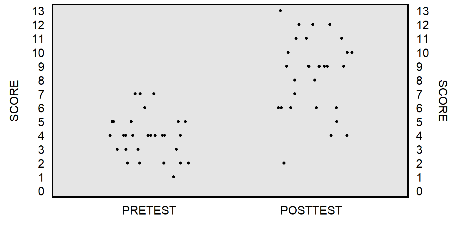
Let’s use data from a prior section of POL 138, in which students at the start of the semester took a 13-item multiple-choice pretest, and then, at the end of the semester, students took the same 13-item multiple-choice test as a posttest. The unpaired t-test will compare the mean pretest score to the mean posttest score, without regard for matching pretest scores to posttest scores for each student:
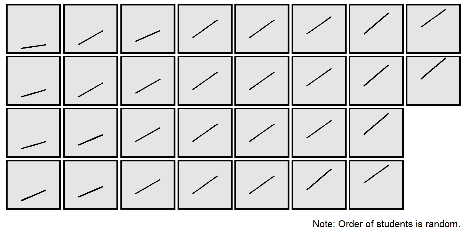
The paired t-test will instead match the pretest score for each student to the posttest score for that student to get a pretest-to-posttest change in score for each student, and then test whether the mean pretest-to-posttest change in scores equals zero:
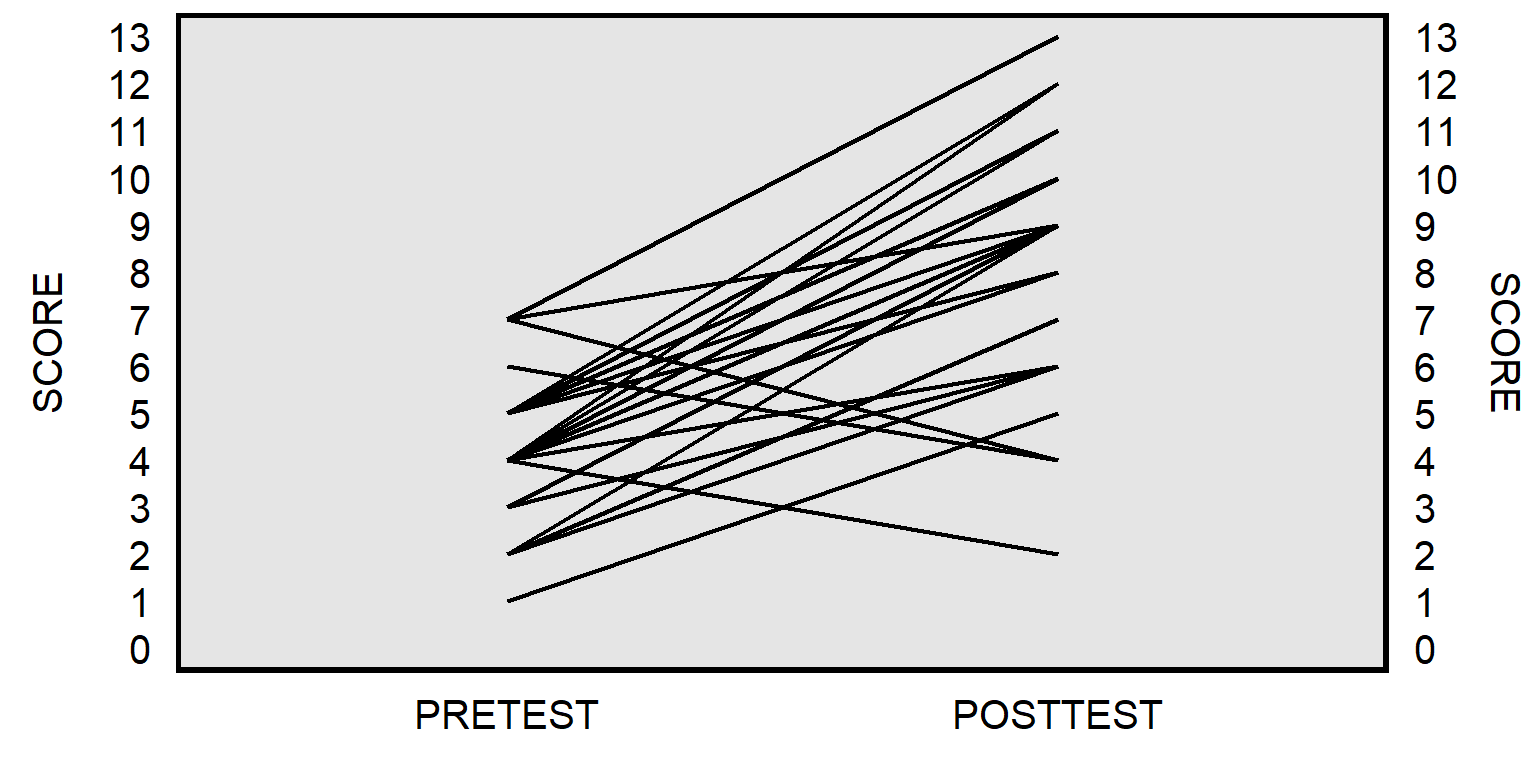
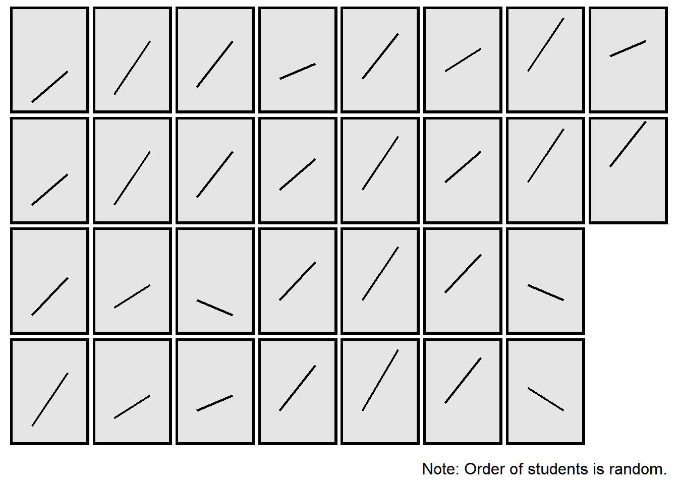
The plot above isn’t ideal because the line for one student might be on top of the line for another student, if multiple students had the same pretest score and posttest score. Below is a better representation, by student:
Below is an R command to conduct an unpaired t-test:
PRETEST  <- c(1,2,2,2,2,2,3,3,3,3,4,4,4,4,4,4,4,4,4,4,5,5,5,5,5,5,6,7,7,7)
POSTTEST <- c(5,6,7,9,9,9,6,6,9,9,2,6,6,8,9,10,10,11,11,12,8,9,10,11,12,12,4,4,9,13)
t.test(PRETEST, POSTTEST, paired = FALSE)
##
## Welch Two Sample t-test
##
## data: PRETEST and POSTTEST
## t = -7.712, df = 46.19, p-value = 0.0000000007682
## alternative hypothesis: true difference in means is not equal to 0
## 95 percent confidence interval:
## -5.548312 -3.251688
## sample estimates:
## mean of x mean of y
## 4.0 8.4Below is an R command to conduct a paired t-test:
PRETEST  <- c(1,2,2,2,2,2,3,3,3,3,4,4,4,4,4,4,4,4,4,4,5,5,5,5,5,5,6,7,7,7)
POSTTEST <- c(5,6,7,9,9,9,6,6,9,9,2,6,6,8,9,10,10,11,11,12,8,9,10,11,12,12,4,4,9,13)
t.test(PRETEST, POSTTEST, paired = TRUE)
##
## Paired t-test
##
## data: PRETEST and POSTTEST
## t = -8.4267, df = 29, p-value = 0.000000002755
## alternative hypothesis: true mean difference is not equal to 0
## 95 percent confidence interval:
## -5.467923 -3.332077
## sample estimates:
## mean difference
## -4.4The p-value for the unpaired t-test (p=0.0000000007682) is lower than the p-value for the paired t-test (p=0.000000002755), indicating that the unpaired analysis provided more evidence against the corresponding null hypotheses than the paired analysis provided. But the p-value for an unpaired t-test will not always be lower than the p-value for a paired t-test: it depends on whether the pairing of the observations produces more or less evidence against the null hypothesis.
For the analysis below, I kept the pretest scores and posttest scores the same, but I shuffled the pairings, so that the pretest-to-posttest change more consistently indicated improvement from pretest to posttest:
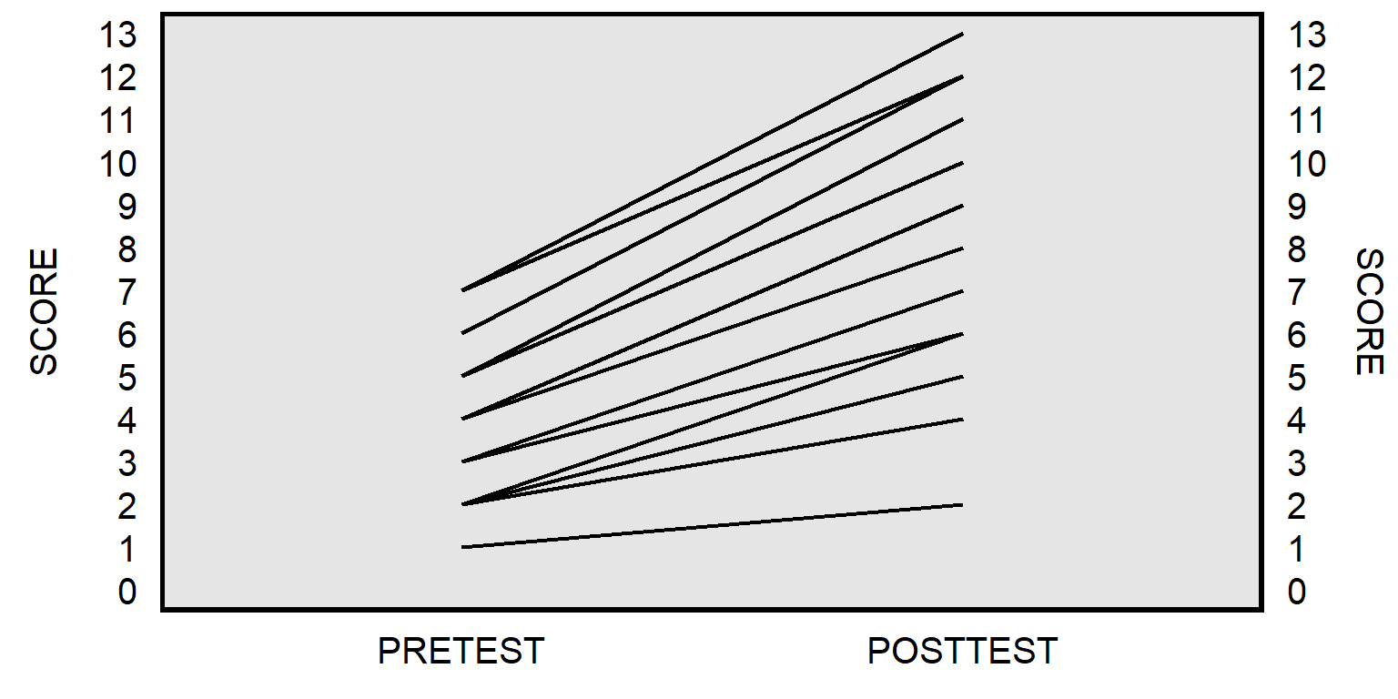
PRETEST.ORIGINAL  <- c(1,2,2,2,2,2,3,3,3,3,4,4,4,4,4,4,4,4,4,4,5,5,5,5,5,5,6,7,7,7)
POSTTEST.SHUFFLED <- c(2,4,4,5,6,6,6,6,6,7,8,8,9,9,9,9,9,9,9,9,10,10,10,11,11,11,12,12,12,13)

t.test(PRETEST.ORIGINAL, POSTTEST.SHUFFLED, paired = FALSE)
##
## Welch Two Sample t-test
##
## data: PRETEST.ORIGINAL and POSTTEST.SHUFFLED
## t = -7.712, df = 46.19, p-value = 0.0000000007682
## alternative hypothesis: true difference in means is not equal to 0
## 95 percent confidence interval:
## -5.548312 -3.251688
## sample estimates:
## mean of x mean of y
## 4.0 8.4##
## Paired t-test
##
## data: PRETEST.ORIGINAL and POSTTEST.SHUFFLED
## t = -18.502, df = 29, p-value < 0.00000000000000022
## alternative hypothesis: true mean difference is not equal to 0
## 95 percent confidence interval:
## -4.886368 -3.913632
## sample estimates:
## mean difference
## -4.4In this case, the p-value for the unpaired t-test is still p=0.0000000007682. But the p-value for the paired t-test is even smaller.
Some statistical tests produce p-values that are approximations, so it’s a good idea to check the assumptions of the test before using the test. For example, an assumption of a two sample t-test is that the data in each sample are distributed normally.
Sample practice items
Among the 30 students in a POL 138 section who took the multiple-choice pretest at the start of the semester and then took the same multiple-choice test as a posttest at the end of the semester, the mean pretest score was 4.0, the mean posttest score was 8.4, and the p-value was p<0.05 for an unpaired t-test of the null hypothesis that the mean pretest score equals the mean posttest score. Is this sufficient evidence at the conventional level in political science to conclude that, at least on average, these students learned something about the POL 138 content on the test?
- Yes
- No
Answer
- Yes
There are two possible explanations for the difference between the 4.0 pretest mean score and the 8.4 posttest mean score: [1] the students on average learned more about the POL 138 content, and [2] the students by random luck happened to guess more correct responses on the posttest than on the pretest. But the p-value under p=0.05 permits us to eliminate random guessing as a plausible explanation at the conventional level in political science, so the only other plausible explanation is that the students on average learned more about the POL 138 content.
14.5 Review
There are a lot of statistical tests, but we will focus on the tests below and their potential uses:
| TEST | EXAMPLE OF USE |
|---|---|
| Binomial test | Comparing a sample percentage to particular percentage. |
| Fisher’s exact test | Comparing a sample percentage to another sample percentage. |
| One sample t-test | Comparing a sample mean to a particular mean. |
| Two sample t-tests | Comparison of the mean from one sample to the mean of another sample. |
Sample practice items
Suppose that we randomly sample 120 residents from a state, and 30 of these state residents indicate that they are members of the Democratic Party and 40 of these state residents indicate that they are members of the Republican Party. Of the tests below, which test would be most appropriate for testing the null hypothesis that the percentage of Democratic Party residents in the state equals the percentage of Republican Party residents in the state?
- binomial test
- Fisher’s exact test
- one-sample t-test
- two-sample t-test
Answer
- Fisher’s exact test
Suppose that we pull a random sample of 30 jelly beans from a jar, and 10 of these jelly beans are red. Which test below would be more appropriate for testing the null hypothesis that the percentage of red jelly beans in the jar is 20%?
- binomial test
- Fisher’s exact test
- one-sample t-test
- two-sample t-test
Answer
- binomial test
Suppose that, in a particular state, we randomly sample 100 men and 100 women, and – on a scale from 0 for very liberal to 10 for very conservative – the mean political ideology of these men is 5.8 (standard deviation of 3.2) and the mean political ideology of these women is 3.9 (standard deviation of 2.8). Which test below would be more appropriate for testing the null hypothesis that the mean political ideology of men in the state equals the mean political ideology of women in the state?
- binomial test
- Fisher’s exact test
- one-sample t-test
- two-sample t-test
Answer
- two-sample t-test
Suppose that we randomly sample 120 residents from a state, and 30 of these state residents indicate that they are members of the Democratic Party. Which test below would be more appropriate for testing the null hypothesis that the percentage of Democratic Party residents in the state is 40%?
- binomial test
- Fisher’s exact test
- one-sample t-test
- two-sample t-test
Answer
- binomial test
Suppose that we randomly sample 200 residents from a state, and the mean political ideology of these residents is 4.1, on a scale from 0 for very liberal to 10 for very conservative. Which test below would be more appropriate for testing the null hypothesis that the mean political ideology of residents in the state is 5?
- binomial test
- Fisher’s exact test
- one-sample t-test
- two-sample t-test
Answer
- one-sample t-test
Suppose that we randomly sample 100 residents of a state. Among these residents, on a 0-to-100 scale, the mean rating about the Democratic Party is 65 (standard deviation of 12) and the mean rating about the Republican Party is 43 (standard deviation of 18). Which test below would be more appropriate for testing the null hypothesis that state residents rate the Democratic Party equal to how they rate the Republican Party?
- binomial test
- Fisher’s exact test
- one-sample t-test
- two-sample t-test
Answer
- two-sample t-test