7 Non-random comparisons
7.1 Discontinuity designs
Major learning objective(s) for this section:
- Explain the logic of a discontinuity design.
A discontinuity design compares observations just below a threshold that received a treatment, to observations just above the threshold that did not receive the treatment. The presumption is that, compared to observations just below the threshold, observations just above the threshold are reasonably similar on all relevant characteristics other than receiving the treatment, so that the only major difference between the groups is the receipt of the treatment.
For example, suppose that we are interested in whether a college student being assigned to an honors program at that college increases that student’s income in their first year after college. Let’s illustrate this below, with hypothetical data for students at a college in which each student who has a 3.0 GPA or higher is in the honors program and no other student at the college is in the honors program. The red dots represent the students who have a GPA below 3.0 and who are thus not in the honors program, and the green dots represent the students who have a GPA of 3.0 or higher and who are thus in the honors program…
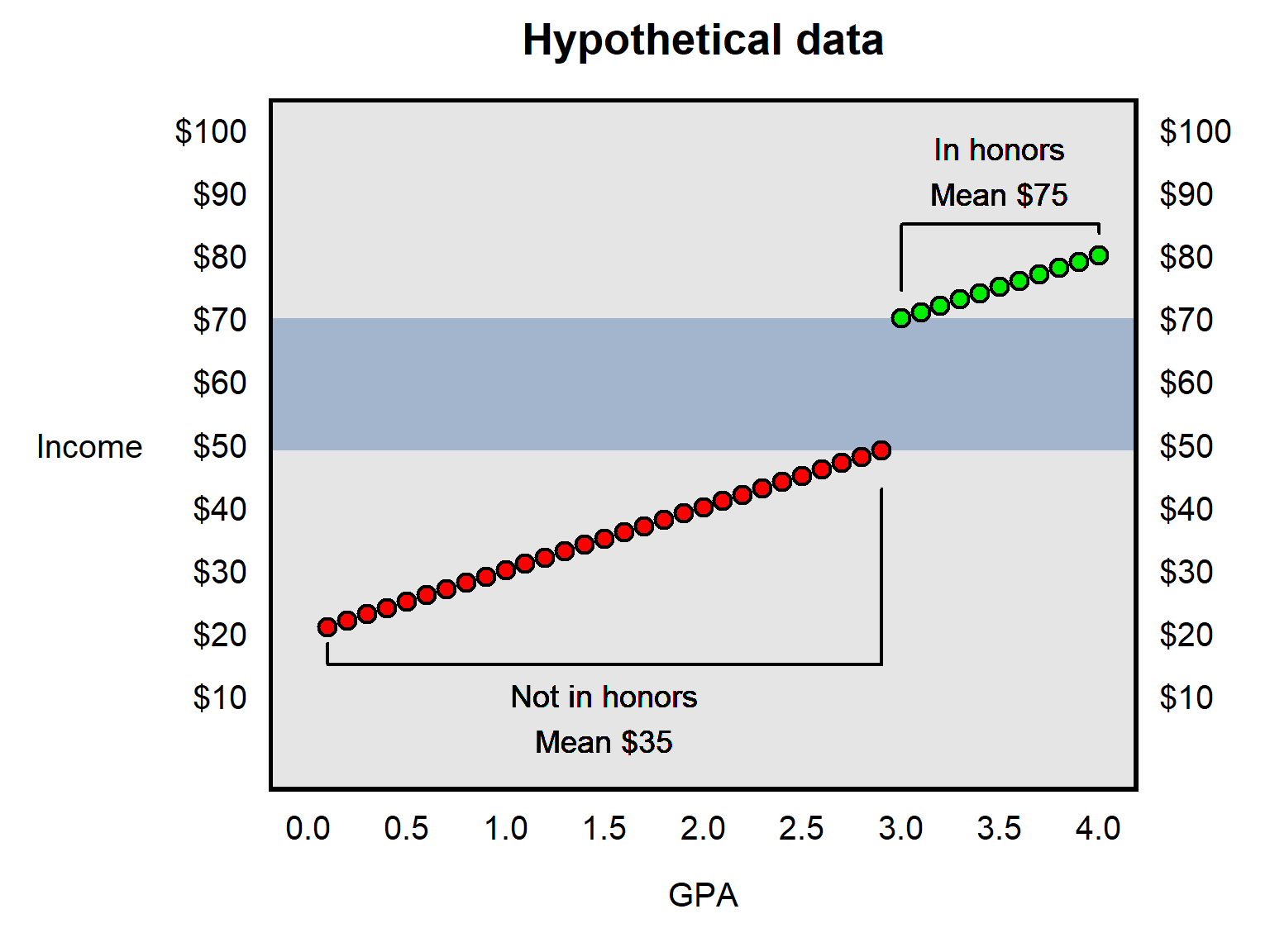
One bad way to estimate the effect of being in the honors program is to compare the mean income for the honors students ($75) to the mean income for the non-honors students ($35) and then estimate that the effect of the honors program is a $40 increase in income. This flaw in that reasoning is that a lot of that $40 gap might be attributed to factors other than the honors program; for example, in our hypothetical, the mean GPA is about 3.5 among honors students and only about 1.5 among non-honors students, so maybe the $40 gap is due to factors such as intelligence and conscientiousness that might cause student differences in GPA.
For a discontinuity design, we might instead compare the income among students who were just below the threshold to get into the honors program ($49, in our hypothetical, at a 2.9 GPA) to the income among students who were just above the threshold to get into the honors program ($70, in our hypothetical, at a 3.0 GPA), to estimate that the effect of the honors program is about a $21 increase in income. The logic of this more restricted comparison is that – other than being in a honors program – a non-honors student with a 2.9 GPA is presumably relatively similar on all relevant factors to a honors student with a 3.0 GPA, compared to how similar a typical non-honors student is to a typical honors student.
The discontinuity design has the advantage of being able to produce a plausible estimate of the treatment effect. But the limitation is that this estimate of the treatment effect is local to the threshold. In our example above, the discontinuity design will provide a plausible estimate of the effect of being in the honors program among students around the threshold for getting into the honors program. But this estimate isn’t necessarily a plausible estimate of the treatment effect on students far from the threshold.
For another example of a discontinuity design, consider the Kuipers 2022 article “Failing the Test: The Countervailing Attitudinal Effects of Civil Service Examinations”:
I surveyed the universe of recent applicants to the Indonesian civil service to study the effects of high-stakes examinations on political attitudes. Leveraging applicants’ scores on the civil service examination, I employ a regression discontinuity design to compare the attitudes of applicants who narrowly failed with those who narrowly passed. I show that the simple fact of failure on the civil service examination decreased applicants’ belief in the legitimacy of the process and levels of national identification while increasing support for in-group preferentialism.
Sample practice items
Redlining is the practice of discriminating against persons who live in “redlined” areas, such as not lending money to persons who live in redlined areas. Many redlined areas in the United States have been areas in which Blacks were disproportionately represented. Suppose that we wanted to estimate the extent to which redlining has reduced the wealth of persons who currently live in redlined areas. Explain which of these two research designs would be better:
- Compare the average wealth of contemporary U.S. residents who currently live in redlined areas, to the average wealth of contemporary U.S. residents who do not currently live in redlined areas.
- Compare the average wealth of contemporary U.S. residents who currently live at the edge of a redlined area inside the redlined area, to the average wealth of contemporary U.S. residents who currently live at the edge of a redlined area outside the redlined area.
Answer
(B), to hold more factors similar to each other.Researcher A and Researcher B plan to estimate the effect, if any, that getting married has on quarterback performance in the National Football League. Researcher A plans to compare, for each quarterback that has ever been married while in the NFL, that quarterback’s rating over that player’s NFL career before getting married to that quarterback’s rating over that player’s NFL career after getting married. Researcher B instead plans to compare, for each quarterback that has ever been married while in the NFL, that quarterback’s rating only in the player’s NFL *season* before getting married to that quarterback’s rating only in the player’s NFL *season* after getting married. Researcher A claims that his research design is better because his effective sample size is larger than Researcher B’s effective sample size, because Researcher A’s research design will include more years for the quarterbacks. Does Researcher B’s research design have any advantage over Researcher A’s research design? If so, what is that advantage?
Answer
Researcher A’s research design to compare multiple years before and after getting married means that the effect of marriage will be reasonably strongly associated with the effect of being older, because older players will be more likely to be married. Therefore, if quarterbacks have a drop off in performance after getting married, we won’t know whether that is because of age or because of being married. Researcher B’s research design reduces the potential for this to be a problem, because Researcher B will be comparing players only one season apart.7.2 Difference-in-differences designs
Major learning objective(s) for this section:
- Explain the logic of a difference-in-differences design.
Like a discontinuity design, a difference-in-differences design can be used when there is a major break in which it is plausible that the break is the only major change and thus can be considered as if it were an experimental treatment. But a difference-in-differences design includes a comparison group that, before the treatment, was similar to the group of interest and, as best we can tell, should be expected to have been similar to the treated group afterwards, if not for the difference in treatment.
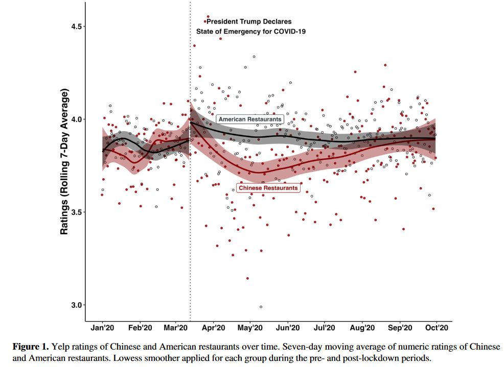
For example, the plot below from Kim and Kam 2023 indicates that, after the covid-19 emergency was declared, Yelp reviews about Chinese restaurants decreased; this seems plausibly due to anti-Chinese sentiment, because of claims that covid came from China. But the decrease is Yelp ratings for Chinese restaurants might not be particular to Chinese restaurants. After the covid declaration, most restaurants transitioned to delivery, so maybe all restaurants experienced a drop in Yelp ratings, if Yelp raters merely didn’t like eating delivery as much as eating in person. Kim and Kam 2023 addressed that potential alternate explanation by comparing the difference in Yelp ratings about Chinese restaurants before and after the covid-19 emergency was declared, to the difference in Yelp ratings about American restaurants before and after the covid-19 emergency was declared. The decrease in Yelp ratings for Chinese restaurants did not occur for American restaurants, which can give us more confidence that that decrease in Yelp ratings for Chinese restaurants was due to anti-Chinese sentiment.
Sample practice items
Suppose that, in 2010, 2011, and 2012, economic growth was 3% per year in Freedonia and was 3% per year in neighboring Oceania. On 1 January 2013, Freedonia changed its economic policy, and in 2013, 2014, and 2015 (the most recent year for which data is available), the economic growth rate was 4% per year. One way to estimate the effect, if any, of the effect of the change in Freedonia’s economic policy on Freedonia’s economic growth is to compare the 3% economic growth before the change to the 4% economic growth after the change. But an even better method can be to compare the 1% difference in economic growth in Freedonia before and after 1 January 2013 to the difference in economic growth in Oceania before and after 1 January 2013. Explain a benefit of using the before/after difference in Oceania to help estimate the effect of Freedonia’s 1 January 2013 change in its economic policy.
Answer
The comparison to Oceania helps isolate whether any difference is particular to Freedonia.Suppose that, on 1 January 2018, Freedonia City put into effect a law that banned prostitution. We want to estimate how this ban affected drug crime. Before the prostitution ban, drug crime in Freedonia City had been increasing at 3% per year, but, after the prostitution ban, drug crime in Freedonia City increased at only 1% per year. Like Freedonia City, Otisburg and Luthorville are cities in Freedonia. Prostitution was legal in Otisburg and in Luthorville before and after 1 January 2018. For estimating how the Freedonia City ban on prostitution affected drug crime in Freedonia City, which of these cities would provide the better comparison for a difference-in-difference design, based on the information below?:
- Otisburg, in which drug crime was increasing at 3% per year before 1 January 2018
- Luthorville, in which drug crime was increasing at 3% per year after 1 January 2018
Answer
- Otisburg, in which (like in Freedonia City) drug crime was increasing at 3% per year before January 1, 2018
Suppose that a researcher is interested in the extent to which college causes persons to become more liberal politically. In 2019, the researcher surveys a representative sample of age-18 persons who attend college and a representative sample of age-18 persons who do not attend college; four years later, in 2023, the researcher surveys each person again. Suppose that the researcher’s data is as in the table below, in which political ideology is measured from 0 for extremely liberal to 10 for extremely conservative.
| Group | Mean ideology at age 18 | Mean ideology at age 24 |
|---|---|---|
| Persons in college | 4.5 | 3.5 |
| Persons not in college | 5.0 | 4.2 |
If the researcher analyzed only the data for persons in college, the researcher’s (incorrect) estimate of the effect of college on the political ideology of persons in the researcher’s sample would be that college…
- made persons in the sample about 0.2 units more liberal on average
- made persons in the sample about 0.8 units more liberal on average
- made persons in the sample about 1.0 unit more liberal on average
- made persons in the sample about 3.5 units more liberal on average
Answer
- made persons in the sample about 1.0 unit more liberal on average
Suppose that a researcher is interested in the extent to which college causes persons to become more liberal politically. In 2019, the researcher surveys a representative sample of age-18 persons who attend college and a representative sample of age-18 persons who do not attend college; four years later, in 2023, the researcher surveys each person again. Suppose that the researcher’s data is as in the table below, in which political ideology is measured from 0 for extremely liberal to 10 for extremely conservative.
| Group | Mean ideology at age 18 | Mean ideology at age 24 |
|---|---|---|
| Persons in college | 4.5 | 3.5 |
| Persons not in college | 5.0 | 4.2 |
If the researcher used a difference-in-differences design that compared persons in college to persons not in college, the researcher’s (more correct) estimate of the effect of college on the political ideology of persons in the researcher’s sample would be that college…
- made persons in the sample about 0.2 units more liberal on average
- made persons in the sample about 0.8 units more liberal on average
- made persons in the sample about 1.0 unit more liberal on average
- made persons in the sample about 3.5 units more liberal on average
Answer
- made persons in the sample about 0.2 units more liberal on average
7.3 Benchmarks
Major learning objective(s) for this section:
- Discuss the quality of a benchmark in the political science context.
One of the most important questions to ask when assessing data is: “Compared to what?”. A benchmark is a comparison that we can use to address the “compared to what?” question. For example, the Washington Post maintains a database of fatal police shootings that have occurred in the United States since the start of 2015. In Summer 2020, the database had 5,429 entries, in which each entry was a person fatally shot by police. Below is the percentage fatally shot by police, by gender:
| Gender | % of the U.S. population | % fatally shot |
|---|---|---|
| Female | 50% | 4% |
| Male | 50% | 96% |
Men are about 50 percent of the U.S. population, so men are extremely over-represented among persons fatally shot by police. But, before we conclude that police have unfairly been more likely to fatally shoot men than women, we might consider alternate explanations other than gender bias. For instance, compared to women suspects, men suspects might be more likely to flee from police or be more likely to attack police and thus, in a sense, men might be more likely to deserve to be fatally shot, in a world in which police did not have gender bias. Below are some potential benchmarks for assessing whether men are unfairly overrepresented among persons fatally shot by police, such as the percentage of each group among…
- the U.S. population
- the prison population
- persons who resist arrest
- criminal suspects
- criminal suspects who fire a weapon at police
It might not be possible to get an ideal benchmark, but we might be able to get several reasonably good benchmarks that can inform us about the amount, if any, of gender bias in fatal police shootings. If inferences from all plausible benchmarks suggest gender bias, that might be sufficient evidence for us to accept the claim about gender bias in fatal police shootings.
Sample practice items
Suppose that, at a particular airport, security has the option to search or to not search passenger luggage. The country that the airport is in has seen, over the past generation, a relatively large influx of young ethnic minority persons from other countries. Researchers want to assess whether security at this airport has been unfairly biased against ethnic minority passengers, and the researchers have data that indicate that, of all passengers that have been searched, 40% of the passengers have been ethnic minority.
Researcher A suggests that a good benchmark for assessing bias against ethnic minorities in the searches is the percentage of all airport passengers that are an ethnic minority. Researcher B cites data indicating that, within racial and ethnic groups, younger people age 18 to 29 are more likely to have illegal material in their luggage than older people are, so a better benchmark is the percentage of all airport passengers aged 18 to 29 that are ethnic minority.
Indicate which of the two benchmarks is better, and then explain why.
Answer
Researcher B has a better benchmark. Security acting fairly would presumably search more young passengers than old passengers, so that would mean that a higher percentage of ethnic minority passengers would be fairly searched compared to the percentage of non-ethnic-minority passengers. Researcher B’s benchmark would help address the age explanation and thus better isolate any unfair bias that is due to ethnic minority status. The idea is that, in the absence of bias against ethnic minorities, there is a fair reason to search younger passengers, so we need a benchmark that can help better separate the effect of being young from the effect of being an ethnic minority.Suppose that, in a particular country, the minimum age for driving is 16 years of age, and the minimum age for drinking alcohol is 21 years of age. Researchers A and B want to estimate the effect of drinking alcohol on car accidents.
Researcher A plans to compare two numbers:
- the rate of car accidents per mile driven among all persons in the country age 16 through 20, and
- the rate of car accidents per mile driven among all persons in the country age 21 and older.
Researcher B plans to compare two numbers:
- the rate of car accidents per mile driven among all persons in the country age 19 and 20, and
- the rate of car accidents per mile driven among all persons in the country age 21 and 22.
Researcher A tells Researcher B that Researcher B’s research design is worse because Researcher B has a smaller sample size. Research B responds by proposing a benefit of limiting the analysis in this case to two years before the age 21 threshold (19 and 20) and two years after the age 21 threshold (21 and 22). Explain this benefit.
Answer
On average, young drivers are much more likely to be in a car accident than older drivers are. Researcher B’s comparison groups are more similar to each other in age than Researcher A’s comparison groups are, so that helps address the alternate explanation that any difference between comparison groups is not due to alcohol but is due to age.A 2021 report from the National Fire Protection Association indicated that, in homes in the United States between 2014 and 2018, there were 2,620 civilian deaths due to fire. The majority of these deaths due to fire (59%) were in a home that had a smoke alarm. Moreover, the majority of fires (74%), the majority of property damage due to fire (74%), and the majority of civilian injuries due to fire (70%) occurred in U.S. homes that had a smoke alarm. Discuss whether these data indicate that, at least in U.S. homes between 2014 and 2018, U.S. homes would have been safer without a smoke alarm.
Answer
Almost all U.S. homes have a smoke alarm: about 96% in 2010, according to Table 12 in the aforementioned report. Therefore, if smoke alarms had no effect, all else equal, about 96% of deaths due to fire would be in U.S. homes that had a smoke alarm. If having a smoke alarm was more dangerous than not having a smoke alarm, then, all else equal, more than 96% of civilian deaths due to fire would be in U.S. homes that had a smoke alarm. But only 59% of civilian deaths due to fire were in U.S. homes that had a smoke alarm.7.4 Panel designs
Major learning objective(s) for this section:
- Explain how panel designs can help with causal identification.
In cross-sectional data, cases are observed once at one point in time, such as if we surveyed 1,000 participants this past Tuesday or if we observed the crime rate in each state in 2022. But for panel data, we have multiple data points for each case, such as a survey of 1,000 participants this past Tuesday and another survey six months from now, or a measure of the crime rate in each state in 2020, in 2021, and in 2022.
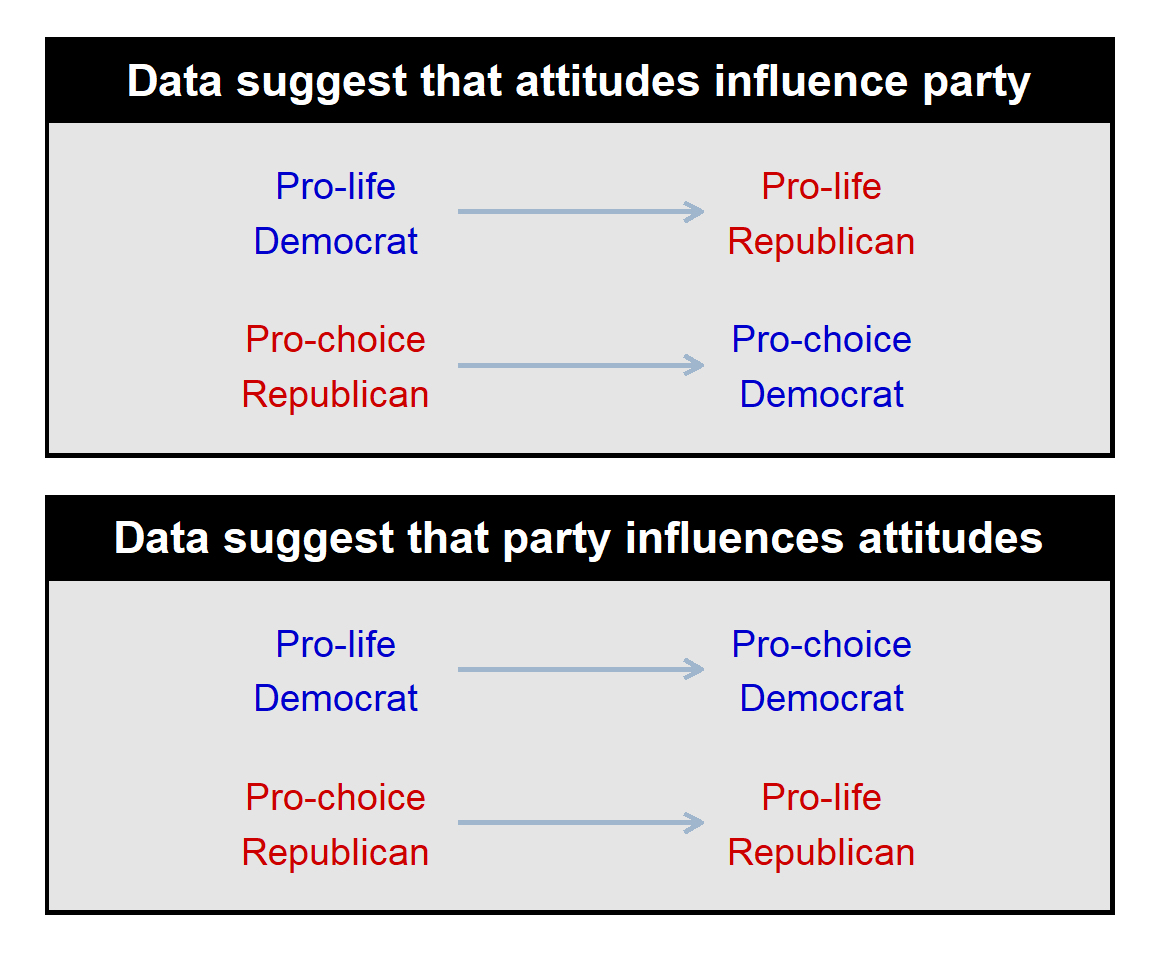
Compared to cross-sectional data, panel data can be more useful for causal identification, because we can observe changes over time within a case. For example, suppose that, compared to a year ago, U.S. residents are now better sorted by partisanship and abortion attitudes, such as if, compared to a year ago, a higher percentage of Republicans are pro-life and a higher percentage of Democrats are pro-choice. Based merely on this pattern, we could not tell whether this is due to a change in party, a change in abortion attitudes, or both. But suppose that panel data indicated that the only relevant changes were pro-life Democrats changing to be pro-life Republicans and pro-choice Republicans changing to be pro-choice Democrats; in that case, we can plausibly infer that abortion attitudes caused these changes in partisanship. But suppose that the panel data instead indicated that the only relevant changes were pro-life Democrats changing to be pro-choice Democrats and pro-choice Republicans changing to be pro-life Republicans; in that case, we can plausibly infer that partisanship caused abortion attitudes to change.
Sample practice items
Suppose that, for four participants, a researcher has data from a survey in January and another survey in December of the same year, with each participant appearing twice in the dataset. For each participant and for both months, the dataset has an indication of the participant’s political party (D or R) and an indication of whether the participant supports or opposes abortion. Data are below, with each participant identified with an ID:
| ID | January | December |
|---|---|---|
| 1 | D + Support | D + Support |
| 2 | D + Oppose | R + Oppose |
| 3 | R + Support | D + Support |
| 4 | R + Oppose | R + Oppose |
Based on these data only, which of the following inference is more supported?
- political party influenced attitudes about abortion
- attitudes about abortion influenced political party