10 Threats to inference 1
Let’s discuss some things that can cause an incorrect inference.
10.1 Selection bias
Major learning objective(s) for this section:
- Discuss how inferences can be biased by selection bias.
- Know what imputation is, for addressing missing data.
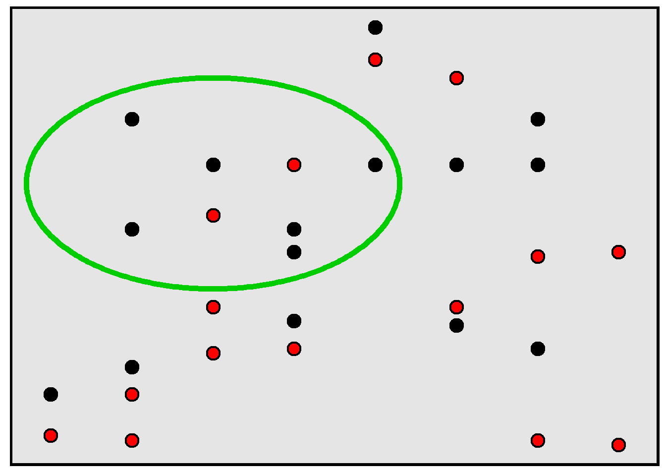
Remember that a population is the set of things of interest for a study, and a sample is the set of things that were studied for the study. Selection bias occurs when a sample is not representative of the population and this causes an incorrect inference about the population. For example, in the rectangle below, 50% of the population of points are red, but, in the sample of points inside the green circle, only 25% of the points are red.
For an example of a potential incorrect inference due to selection bias, suppose that we wanted to estimate the percentage of college students who voted in the most recent election, so we email all college students, asking each student to complete a 50-item survey in which the last item on the survey is an item asking students to report whether they voted in the most recent election. It’s plausible that the percentage of college students who indicated on the survey that they voted in the most recent election is an overestimate of the true percentage of college students who voted in the most recent election, because it’s plausible that the college students who completed the survey are more conscientious on average than other college students and that more conscientious college students are more likely to vote than less conscientious college students are to vote.
Researchers can address an unrepresentative sample by using weights. Researchers can also address missing responses by using imputation, which involves the researcher taking a best guess (or guesses) about what the missing data would have been if the data was not missing. This best guess might be based on data that the researcher has about the observation that had the missing data; for example, if a participant does not indicate their family income, then a researcher might impute a family income for that participant, with the imputed value reflecting the researcher’s best guess at the participant’s income using other data that the researcher knows about the participant, such as the participant’s education level, age, gender, race, and marital status. So if a 40-year-old married Black woman with a college degree does not indicate her family income, we could impute that family income based on the expected family income for a typical 40-year-old married Black woman with a college degree.
Sample practice items
Suppose that Amy taught a section of POL 138 and required student attendance, and Bob taught a section of POL 138 and did not require student attendance. Explain how the difference in attendance policies might cause the instructors to receive different mean ratings for in-person course evaluations conducted on the next-to-last class meeting before the final exam, even if both taught equally well.
Answer
Bob not requiring attendance plausibly means that students who come to class and thus respond to the in-person course evaluations like Bob or like the POL 138 material and thus are plausibly going to provide more positive course evaluations, compared to students who do not come to class. But Amy’s requirement for class attendance plausibly means that more of the students who do not like Amy or like the POL 138 material will come to class and will provide relatively negative evaluations. So Amy’s policy of requiring attendance will likely lower the mean rating for her course, compared to Bob’s policy of not requiring attendance.Suppose that 10,000 persons register for an online course about artificial intelligence. On the first day of the course, each student in attendance that day takes a 10-item pretest about artificial intelligence. On the final day of the 15-week course, each student in attendance that day takes a different 10-item posttest about artificial intelligence that is exactly as difficult as the pretest was. Suppose that the mean percentage correct was 40% on the pretest and was 70% on the posttest, with a p-value of p<0.05 for a test of the null hypothesis that these percentages correct equal each other. Explain whether this is sufficient evidence to conclude that the course caused an increase in students’ knowledge about artificial intelligence.
Answer
Not sufficient evidence. Maybe students who didn’t know much about artificial intelligence dropped the course, so that the only students left already knew a lot about artificial intelligence.10.2 Per capita
Major learning objective(s) for this section:
- Calculate a per capita rate.
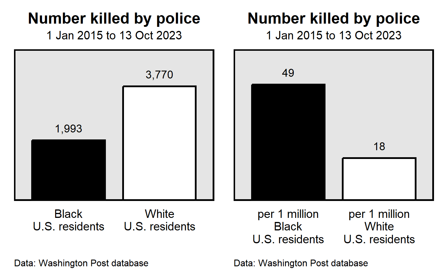
A common threat to inference is the use of absolute numbers when rates are more appropriate. For example, as of 13 Oct 2023, the Washington Post database of fatal police shootings indicated that, since 1 Jan 2015, police in the United States had shot and killed 1,993 Black persons and 3,770 White persons. Police thus shot and killed almost twice as many White persons as police shot and killed Black persons. To the extent that a fatal police shooting is a concern, does this mean that fatal police shootings of White persons is more of a concern than fatal police shootings of Black persons are? Maybe not, if we consider per capita rates, which are rates per person. The United States has about 5 times as many White residents (204 million) as Black residents (41 million), so the rate of fatal police shootings was about 18 per 1 million White persons but was about 49 per 1 million Black persons.
Sample practice items
Data from the U.S. government indicated that the U.S. population has about 64 million Hispanic residents and about 1 million residents who are Native Hawaiian or Pacific Islander and that the year 2019 had 693 single-bias incidents that had a Hispanic victim and 26 single-bias incidents that had a Native Hawaiian or Pacific Islander victim. Based on these data, the number of victims of single-bias incidents was higher among which of the following groups in 2019?
- Hispanic U.S. residents
- Native Hawaiian / Pacific Islander U.S. residents
Answer
- Hispanic U.S. residents
For this item, merely compare the 693 for Hispanics to the 26 for Native Hawaiian or Pacific Islander.
Data from the U.S. government indicated that the U.S. population has about 64 million Hispanic residents and about 1 million residents who are Native Hawaiian or Pacific Islander and that the year 2019 had 693 single-bias incidents that had a Hispanic victim and 26 single-bias incidents that had a Native Hawaiian or Pacific Islander victim. Based on these data, the per capita rate of being a victim of a single-bias incident was higher among which of the following groups in 2019?
- Hispanic U.S. residents
- Native Hawaiian / Pacific Islander U.S. residents
Answer
- Native Hawaiian / Pacific Islander U.S. residents
For this item, the per capita rates are 693/64 million for Hispanics (which is a per capita rate of about 11 per million) and 26/1 million for Native Hawaiian or Pacific Islander (which is a per capita rate of 26 per million).
One concern with measuring the LGBT population is that some LGBT people might be afraid to identify as LGBT. Estimates from the UCLA School of Law Williams Institute were that Idaho has 48,000 residents who identify as LGBT but North Dakota has only 20,000 residents who identify as LGBT. So, compared to North Dakota, Idaho has more than twice as many residents who identify as LGBT. Is this large difference credible evidence that LGBT persons in Idaho are more afraid to identify as LGBT compared to LBGT persons in North Dakota?
Answer
No, because per capita rates are more appropriate to consider. North Dakota has fewer people overall (about 780,000) than Idaho has (about 1.9 million), and the per capita rates of LGBT identification are pretty close to each other: about 2.5 per 100 in Idaho, and 2.6 in North Dakota.10.3 Influential outliers
Major learning objective(s) for this section:
- Know how the influence of outliers can be reduced.
An outlier is data point that is very different from other data points. Such outliers can cause an incorrect conclusion if the outlier is misleadingly influential.
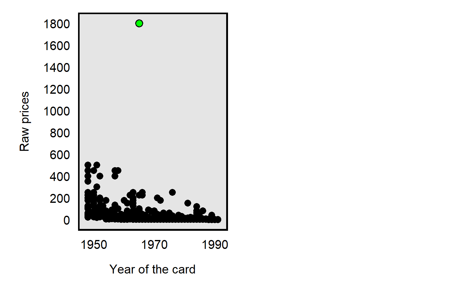
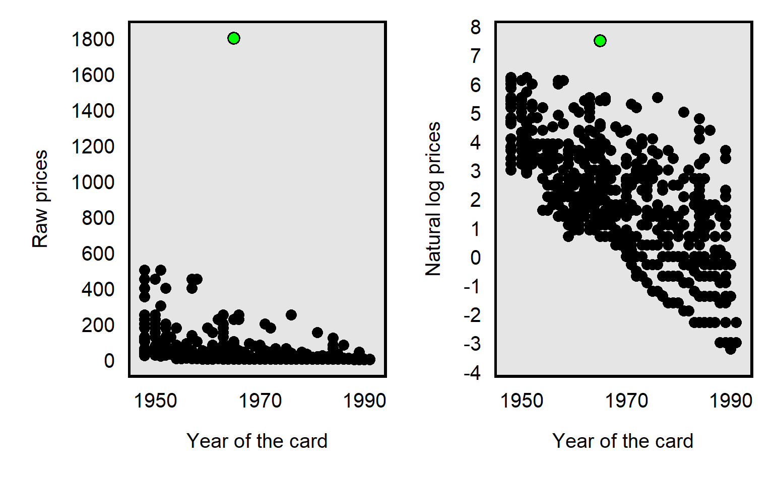
For example, in the dataset for Primm et al 2010 “The Role of Race in Football Card Prices”, the median price for a football card was $3, and the price for all but one football card was $500 or less. However, the football card for Joe Namath was $1,800, which was more than three times as much as the next highest priced card in the dataset, as illustrated in the plot below. So a threat to causal inference would be if Joe Namath’s card is misleadingly influential. Joe Namath is White, so, if our analysis indicated that the cards for White football players were on average priced higher than cards for Black football players were priced, that might be due to unfair bias favoring White players, but we should also assess whether that difference in mean price is due to something distinctive about Joe Namath other than his race.
Researchers have a few ways to deal with outliers, such as:
Conduct the analysis with and without the outlier. For example, for the Joe Namath example of a football card that has an outlier price, we could conduct the analysis including Joe Namath’s card and re-conduct the analysis excluding Joe Namath’s card: if the results are substantially the same, then we can infer that the outlier really doesn’t matter much.
Transform the data so that the outlier is less influential.
One transformation is to reduce the data to categories. For the football card example, instead of measuring the price of football cards to the nearest penny, we could group the cards by price range, such as from 1 cent to 50 cents, 51 cents to 99 cents, $1 to $1.99, and so forth until, say, $300 or more. That way, the Joe Namath card is not all by itself far away from the other cards but is instead in the highest category along with (in this case) 14 other relatively high priced cards. The number of categories and the width of the categories can depend on the amount of data that we have and the usefulness of the categories. This data transformation isn’t ideal, though, because the data transformation loses precision in the measurement, with the $1800 Joe Namath card not being differentiated from the $450 card for Jim Brown or the $300 card for Norm Van Brocklin.
The data transformation that Primm et al 2010 used was the natural log transformation, which pushes numbers together, as illustrated in the plot below, with the Joe Namath card as the green dot:
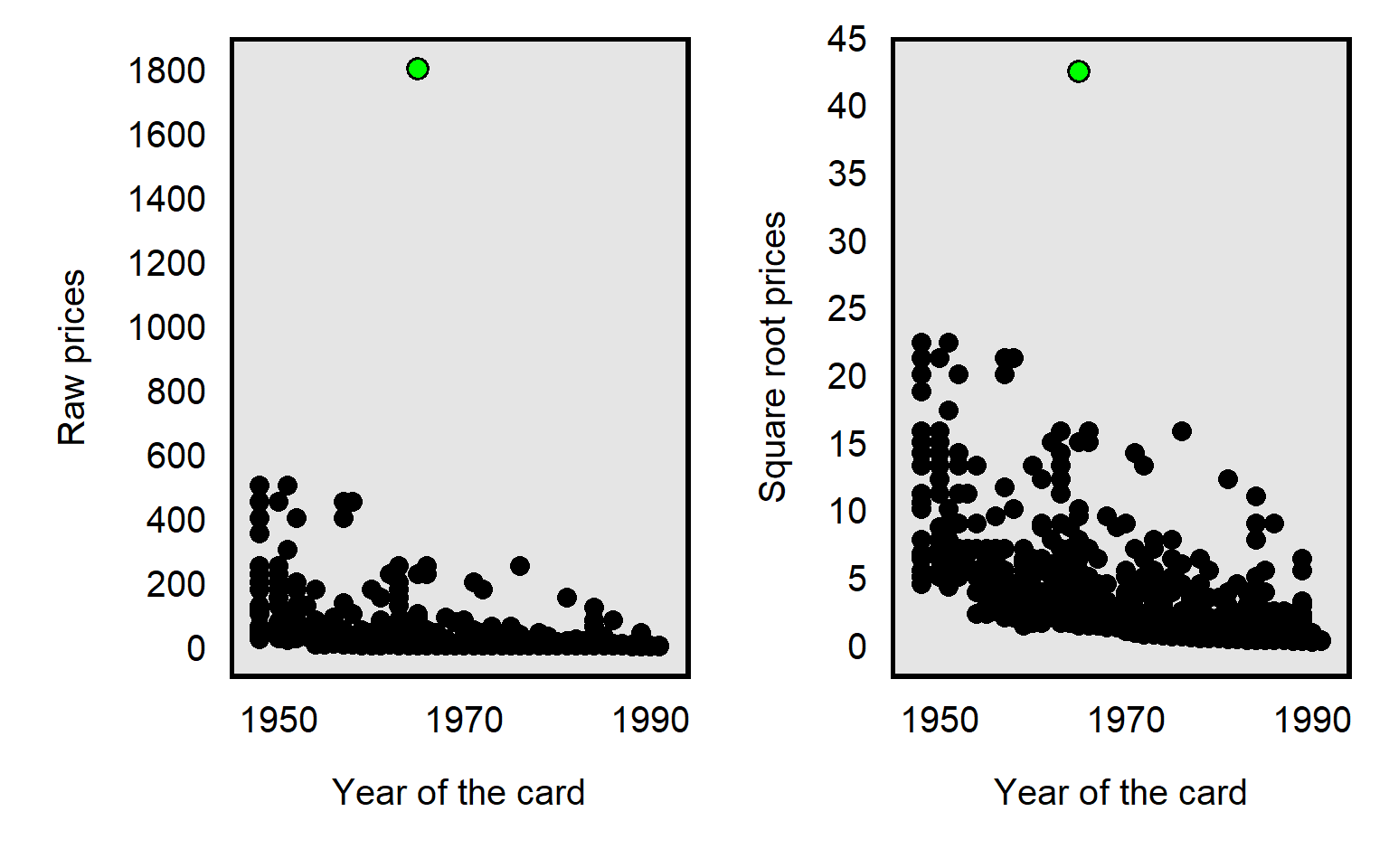
The influence of an outlier can also be reduced by taking the square root the prices, like in the plot below, but, compared to a natural log transformation, the reduction is less extreme for the square root transformation:
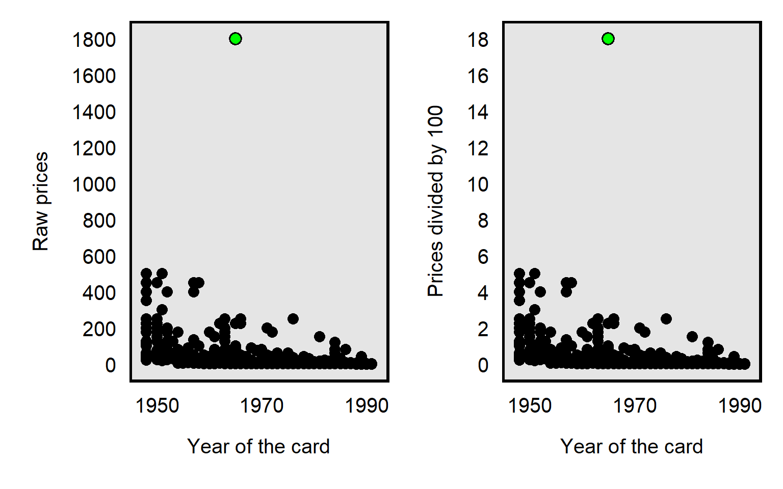
It’s possible to divide each card price by, say, 100, which will reduce the price of the Joe Namath card from $1800 to $18. But dividing by 100 will reduce the price of all cards equally relative to each other, so the dividing by 100 doesn’t affect how influential the outlier is:
Sample practice items
Suppose that a dataset contains annual salaries for 100 respondents, with 99 salaries between $10 per year and $200,000 per year and one outlier salary of $20 million per year. We use the measure of respondent annual salary to predict respondent support for raising taxes. Select ALL of the data transformations listed below that would plausibly reduce the influence of the outlier on our estimates:
- dividing the salaries by 100
- taking the natural log of the salaries
- squaring the salaries
- square rooting the salaries
Answer
- taking the natural log of the salaries
- square rooting the salaries
10.4 Using a less relevant measure
Major learning objective(s) for this section:
- Select and defend a relevant measure for an analysis.
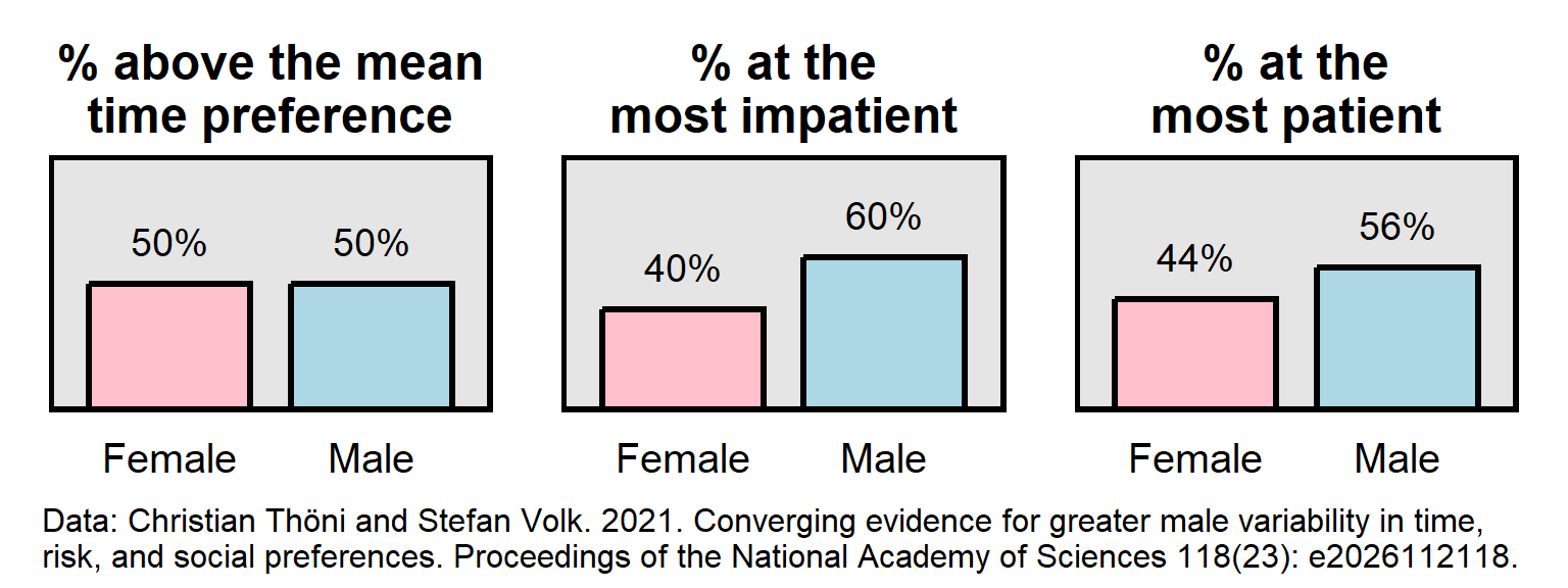
Sometimes the most appropriate measure for an analysis is the mean, and sometimes the most appropriate measure for an analysis is the median. But sometimes the most appropriate measure for an analysis is a percentile at a high end or low end of a set of data.
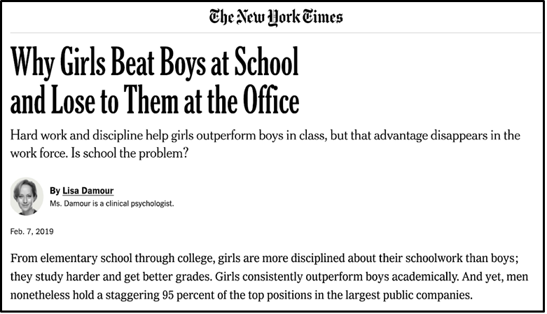
An example of this flaw appeared in the New York Times, in which an author compared boys and girls on average to men and women in top positions in business. But average students don’t tend to become top business executives, so a more relevant comparison would have been to compare gender differences among top business executives to gender differences among top students.
Below is an example of a pattern in which two groups have the same mean on a measurement but are not equally represented at the ends of the distribution of the measurement. In this pattern, the outcome is time preference, which is a measure of patience. In these data, male participants were as patient as female participants were, on average. However, male participants were overrepresented among the most impatient participants and were overrepresented among the most patient participants.
Sample practice items
Suppose that each public high school in Illinois selects their three best math students to represent the school in a competition answering math questions. For each student, we have data on the student’s score on the most recent state standardized math test. Explain which one of the following would be most useful for predicting which school will win the competition:
- the 1st percentile score for each school on the state standardized math tests
- the mean score for each school on the state standardized math tests
- the median score for each school on the state standardized math tests
- the 99th percentile score for each school on the state standardized math tests
Answer
- the 99th percentile score for each school on the state standardized math tests
10.5 Measurement error
Major learning objective(s) for this section:
- Discuss how inferences can be biased by measurement error.
Measurement error occurs when measurements are incorrect. Below are illustrations:
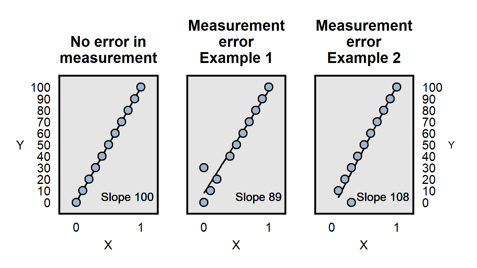
Measurement error can involve incorrect measurement, but imprecise measurement can also be a problem. Imagine, for instance, that a pill really causes participants to lose 10 pounds on average and that we have a measure of participant weight before and after taking the pill. If our measurement of participant weight is merely whether a person is overweight, then we might not have sufficient precision in the measurement of the outcome to detect the true effect of the weight loss pill, if all of the weight loss involves changes such as 250 lbs to 240 lbs, in which both weights are coded as “overweight” and thus there is no change in the measurement.
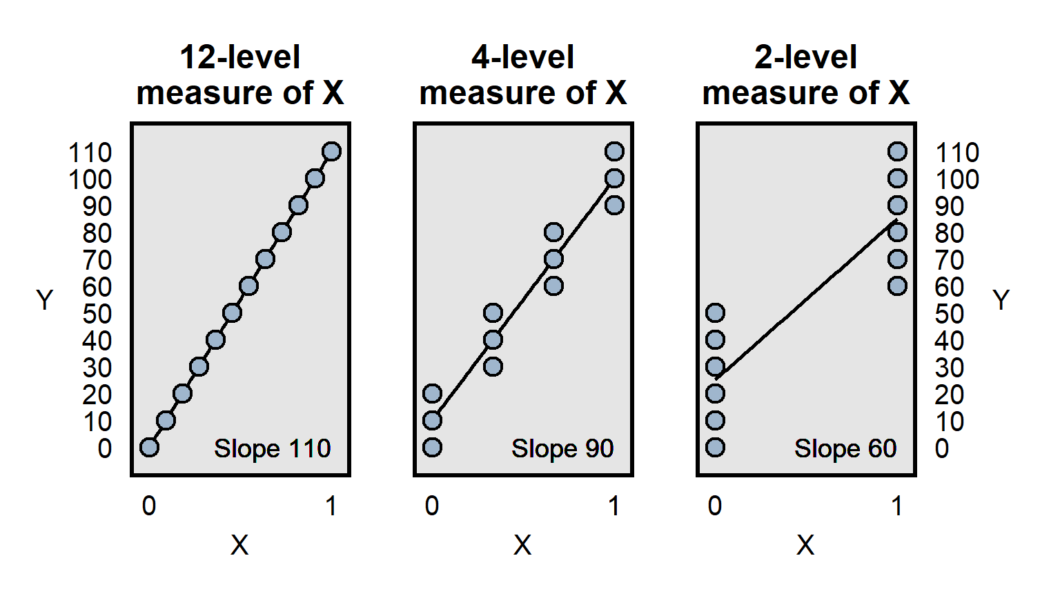
Differences in measurement precision can be a particular problem for analyses that attempt to compare how well predictors predict an outcome, because a predictor that is measured more precisely will, all else equal, have an advantage in that comparison, because the lack of precision is expected to bias estimates toward zero, as illustrated below:
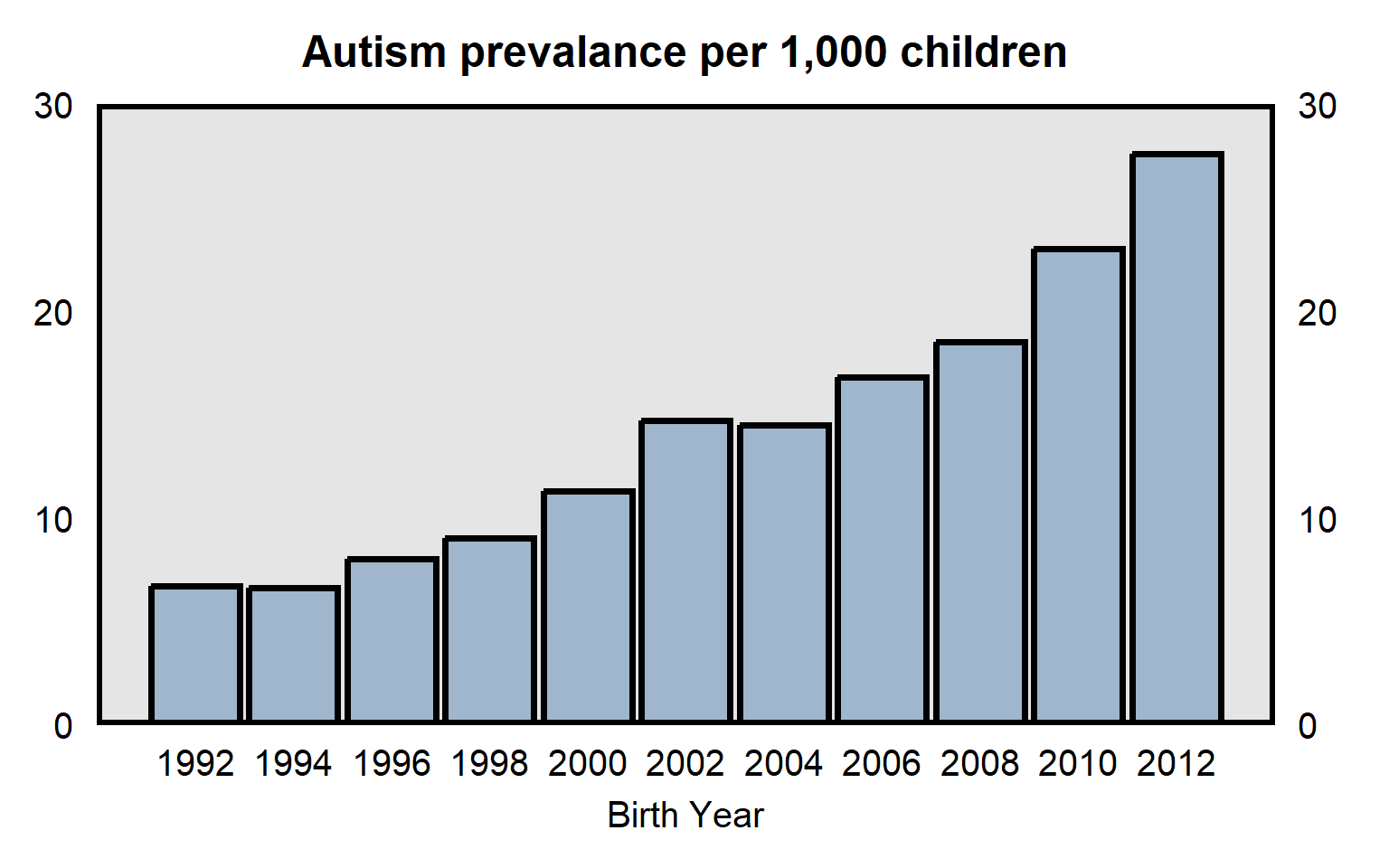
It is useful to consider whether patterns might be influenced by measurement error. For example, data from the Centers for Disease Control and Prevention in the plot below indicates the prevalence of autism among U.S. children born between 1992 and 2012. The substantial increase over time might be due to an increase in the prevalence of autism, but part or all of the increase might be due to changes in the measurement of autism, such as if doctors over time became more likely to diagnose the same set of behaviors as autism.
Sample practice items
Suppose that, over the past ten years, the reported number of burglaries has substantially decreased in Freedonia City. One possible explanation for this is that the prevalence of burglary has dropped. But what else might this be due to?
Answer
One possible response: The decrease in the reported number of burglaries might be due to victims of a burglary being less likely to report the burglary, such as if police over time have become much less likely to sincerely investigate burglaries or much less likely to successfully return stolen goods.Suppose that we assess whether, for predicting support for the president, participant attitudes about immigrants matters more or less than participant attitudes about women. Our measure of participant attitudes about immigrants is one item that has three levels, and our measure of participant attitudes about women is a scale that combines four items about women, each of which has five levels, so that the measure of participant attitudes about women has 21 levels. Therefore, our measure of participant attitudes about women is a higher quality measure than our measure of participant attitudes about immigrants. Suppose that results from our analysis indicate that the correlation between participant attitudes about immigrants and support for the president is stronger than the correlation between participant attitudes about women and support for the president. The fact that the measure of participant attitudes about immigrants is a lower quality measure than our measure of participant attitudes about women should make us ___ that participant attitudes about immigrants truly matters more than and participant attitudes about women, for explaining support for the president.
- less confident
- more confident
Answer
- more confident
Poor measurement in a predictor is expected to bias results toward a null result, so the bias in this case (with the measure of participant attitudes about immigrants being lower quality) should make us more confident that participant attitudes about immigrants truly is a better predictor of the outcome of support for the president.
10.6 Restriction of range
Major learning objective(s) for this section:
- Discuss how inferences can be biased by restriction of range.
Restriction of range is a type of measurement imperfection in which the measure does not extend far enough in some way, to capture the important variation of interest. For example, imagine that we intend to use a 10-item math test to assess whether men have a different math ability than women do, on average.
If the 10 items are so easy that everyone gets all 10 correct, results would indicate that men have the same math ability as women have, but this inference of no gender difference in math ability might merely be because the test was too easy.
If the 10 items are so difficult that no one gets any item correct, results would indicate that men have the same math ability as women have, but this inference of no gender difference in math ability might merely be because the test was too difficult.
For another example, in 2023, all six members of the U.S. team at the International Mathematical Olympiad for high school students were male. If we wanted to assess whether this gender difference is fair, we could try to get a sense of the gender distribution among the very best math students, using data for SAT test takers who scored a perfect on the SAT-Math exam. Below are data from the SAT in 2015, indicating that female test-takers were 33% of the total test-takers who got a perfect score on the SAT-Math test. So shouldn’t we expect about 33% of the members of the U.S. team at the International Mathematical Olympiad to be female?
| Gender | Number of perfect scores | % of the total |
|---|---|---|
| Males | 11,098 | 67% |
| Female | 5,570 | 33% |
Not necessarily: In 2015, the SAT math test had 16,668 perfect scores, so the SAT data can inform us about the gender distribution among the top 16,668 students in math. However, the SAT data can’t inform us about the gender distribution among the top six students in math.
For another example, suppose that one reason why men’s salaries tend to be higher that women’s salaries is because men are more likely to ask for a raise. Suppose that the data indicate only whether men and women have ever asked for a raise at work. If the data indicated that men were just as likely as women to have ever asked for a raise, that would not permit us to infer that asking for a raise is not a cause of the gender pay gap, because it might be that men who ask for a raise ask for a raise more often than women who ask for a raise ask.
Sample practice items
Suppose that I want to test whether the mean level of political knowledge among male students differs from the mean level of political knowledge among female students. I therefore give a political knowledge test to each student in POL 138. The items are all multiple-choice. Sample items are “Who is the current U.S. president?” and “In what year did the War of 1812 begin?”. Suppose that results indicate that there is no gender difference in political knowledge. Explain a potential flaw in this research.
Answer
Ceiling effect. The test items are so simple that, even if male students did differ from female students in their political knowledge, this test is too easy to detect that difference.Suppose that our political knowledge test had 5 extremely easy items and 10 extremely difficult items. Would we still need to worry about restriction of range, such as a floor effect or a ceiling effect?
Answer
Yes. If each person gets all extremely easy item correct, and each person does not get any extremely difficult item correct, then everyone would get the same number correct, and thus we would not be able to detect a difference, even if the difference exists.10.7 Confounders
Major learning objective(s) for this section:
- Discuss how inferences can be biased by not controlling for confounders.
The problem of confounding occurs when the association between a predictor and an outcome is due to a third variable, called a confounder.
Consider the van Boven et al 2006 randomized experiment that tested for racial bias, in which participants were randomly shown only one of the photos below and were asked the item below:

Q11. The person in the photograph is holding several items. To what extent to you agree or disagree that this person is looting?

- Strongly Agree
- Moderately Agree
- Slightly Agree
- Neither Agree nor Disagree
- Slightly Disagree
- Moderately Disagree
- Strongly Disagree
The outcome of participant perceptions about whether the person in the photograph is looting could be influenced by the race of the person in the photograph (and thus be influenced by racial bias), but there are other differences between the photographs that confound that inference. For example, compared to the Black person, the White person seems like he is struggling more because he is carrying more items than he can comfortably carry. Even the difference in what is being carried (wine bottle for the White person only) could be a confound that makes it difficult for the experiment to isolate the effect of the race of the person in the photograph.
For another example, suppose that a class has 100 students, and, before the final exam, 20 of the students attend a study session and the other 80 students don’t attend the study session. Suppose that each of the 20 study session students earns a higher score on the final exam than any of the other 80 students earn. It could be that attending the study session caused the higher final exam scores. But it also could be that something else influenced both whether students attended the study session and the students’ scores on the final exam. For example, maybe conscientiousness caused the 20 study session students to attend the study session and to study for the final exam independently of the study session, so that the 20 study session students would have earned a higher scores on the final exam even without the study session.
Below is a plot from a post at the political science blog called The Monkey Cage (archived). The height of the columns in the plot indicates the percentage of White respondents who opposed paying college athletes. The left column is for White participants who were randomly assigned to not be shown a picture and were then asked to report their feelings about paying college athletes; the right column is for White participants who were randomly assigned to be shown a picture of Black athletes and were then asked to report their feelings about paying college athletes.
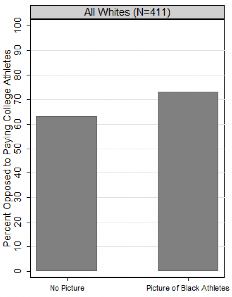
Based on the plot, it might be concluded that racial bias caused opposition to paying college athletes to be higher among White respondents who were shown a picture of the Black athletes. But a research design comparing only these two conditions cannot indicate whether the higher opposition was because the picture had athletes or because the picture had Black athletes. It would have been better to compare the percentage opposition among White participants shown a picture of Black athletes to the percentage opposition among White participants shown a picture of White athletes. That comparison could help us isolate the extent to which a difference in percentage opposition is due to the race of the athletes in the picture.
By the way, the data in the experiment was from a module of the CCES survey, and these modules typically have sample sizes of 1,000 participants. Any guesses why the image reports data for only 411 White participants?
The problem with multiple manipulations per experimental condition can be subtle. Consider the Widner and Chicoine 2011 experiment that involved sending resumes to employers, with the name on the resume randomly assigned to be a stereotypical White name (such as William Novak or James Yoder) or a stereotypical Arab name (such as Abd al-Malik Khalil or Qahhar Kazim). Results from the experiment indicated that the resumes with the stereotypical White name were more likely to receive a callback than resumes with the stereotypical Arab name. The two sets of names differed in the perceived ethnicity of the applicant (White or Arab), but the two sets of names also differed in the degree of difficulty in pronouncing the names in the contemporary U.S. context. It might thus have been better for the experiment to balance the names on this characteristic, such as with difficult-to-pronounce White names (e.g., Pitor Wojciehowicz) or easier-to-pronounce Arab names (e.g., Ahmad Kassab).
For another example, consider a randomized experiment in which participants in one group are asked to recommend a sentence length for a White man who murdered his wife, and participants in the other group are asked to recommend a sentence length for a Black man who murdered his wife. In this case, only one thing has been explicitly changed: the race of the man who murdered his wife. But, because so many marriages are between persons of the same race, many participants might think that the White man murdered a White woman and that the Black man murdered a Black woman. So if the Black man received a lower mean recommended sentence length than the White man received, we could not tell whether that is because participants punished the White man more severely than the Black man or because the participants thought that taking a White woman’s life deserved a more severe punishment than taking a Black woman’s life deserved.
Sample practice items
Statistics indicate that police in the United States made about 18 million traffic stops in 2005. About 61% of these stops were stops of men drivers, and about 39% of these stops were stops of women drivers. The p-value is p<0.05 for a test of the null hypothesis that the percentage of these stops that were stops of men drivers equals the percentage of these stops that were stops of women drivers. Explain whether, based on this evidence and at the conventional level in political science, it should be concluded that police traffic stops in 2005 were unfairly biased against men drivers relative to women drivers.
Answer
No. Men on average might have different driving habits than women, such as speeding or driving more miles, and this difference in driving habits might mean that it is fair for police to make more traffic stops of men than women.10.8 Miscontrolling
Major learning objective(s) for this section:
- Discuss how inferences can be biased by controlling for colliders.
Flawed statistical control might produce an incorrect inference in at least two ways:
Undercontrolling occurs when the analysis is missing a relevant control. For example, if, at a particular company, men are paid more than women on average, that gender difference in payment might be fair if men work more hours on average than women work, so an analysis that does not control for hours worked might produce an incorrect inference that men at that company are unfairly paid more then women at that company.
Overcontrolling occurs when analysis has too many controls, such as controlling for factors that are “downstream” from the predictor that we are interested in. For example, it might be fair for a company to pay workers more if the worker received an award from the company. So an analysis testing for gender bias in worker pay should control for whether the worker received such an award. But there might be gender bias in the decision about which workers are selected to receive an award, so that controlling for receipt of such awards can produce an incorrect inference about gender bias in worker pay if the awards are a mechanism for gender bias in pay.
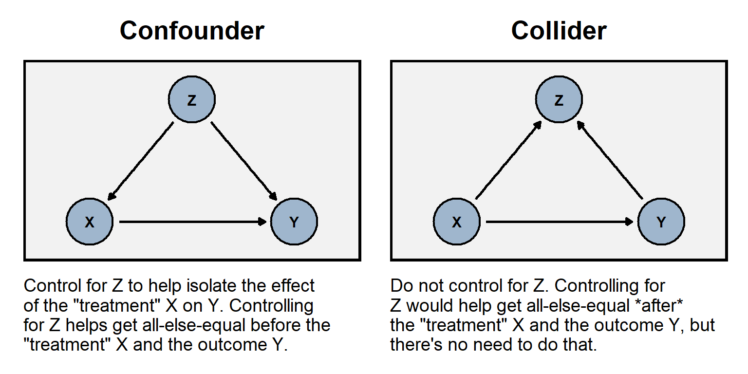
The ideal for control variables is to help get the cases that we are comparing to be equal at the point of the difference in treatment, so that we can estimate the effect of the treatment. Therefore, we want to control for differences that have occurred before the difference in treatment, and we do not want to control for differences that occur because of the difference in treatment.
The plot to the left below illustrates the role of a confounder Z that is “upstream” from a predictor and the outcome; it would be undercontrolling to omit the confounder. The plot to the right below illustrates the role of a collider Z that is “downstream” from a predictor and the outcome; it would be overcontrolling to include the collider.
Like with random assignment error, miscontrolling can bias an estimate to be too low and can bias an estimate to be too high.
For an example of overcontrolling collider bias, consider an analysis of data from a randomized experiment that controls for a factor that is measured after the treatment. For example, suppose that the treatment in an experiment is a campaign ad and that this treatment has two effects: one effect is to make participants more positive about the president, and the other effect is to increase participants’ political interest. Controlling for participant political interest could then bias the estimated effect of the treatment on attitudes about the president. See the table below, with three participants in the control group and three participants in the treatment group, all before receiving the treatment. In this case, the mean political interest is the same in each group, and the mean rating is the same in each group: 70 in the control group, and 70 in the treatment group.
| BEFORE THE TREATMENT | |||
|---|---|---|---|
| Control Group | Treatment Group | ||
| Political Interest | Rating | Political Interest | Rating |
| 4 | 90 | 4 | 90 |
| 3 | 60 | 3 | 60 |
| 3 | 60 | 3 | 60 |
Now check the participants in the table below, after receiving the treatment. The treatment had an effect on the second participant in the treatment group, raising that participant’s political interest to 4 and raising that participant’s rating of the president to 90. The mean of the treatment group has risen to 80.
| AFTER THE TREATMENT | |||
|---|---|---|---|
| Control Group | Treatment Group | ||
| Political Interest | Rating | Political Interest | Rating |
| 4 | 90 | 4 | 90 |
| 3 | 60 | 4 | 90 |
| 3 | 60 | 3 | 60 |
The proper way to analyze the tables is to compare the “after the treatment” control group mean rating of 70 to the “after the treatment” treatment group mean rating of 80 to infer that the treatment has raised the rating by 10 points among these participants. However, if we were to control for participants’ political interest, we would infer that the treatment had no effect, because, at each level of political interest, the mean rating in the treatment group equals the mean rating in the control group.
For a randomized experiment, sometimes researchers control for participant demographics such as race and gender, that are measured before the treatment. This can help reduce uncertainty caused by random assignment error and thus increase the precision of the estimates, which can be a good thing. But researchers sometimes control for participant demographics or other factors that are measured after the treatment, but, as illustrated above, this statistical control can bias estimates if the factors that are measured after the treatment have been affected by the treatment.
Sample practice items
Suppose we test whether variation in X causes variation in Y. Which of the following would be worse to add as a predictor to that regression?
- a variable A that influences X and influences Y
- a variable B that is influenced by X and is influenced by Y
Answer
- a variable B that is influenced by X and is influenced by Y
Suppose that you have a linear regression that attempts to estimate the effect that a predictor has on an outcome. Omitting a control variable that should be included in the regression…
- cannot bias the estimate of the effect of the predictor
- can bias the estimate of the effect of the predictor, but can only bias the estimate toward zero
- can bias the estimate of the effect of the predictor, but can only bias the estimate away from zero
- can bias the estimate of the effect of the predictor, and can bias that estimate toward zero or away from zero
Answer
- can bias the estimate of the effect of the predictor, and can bias that estimate toward zero or away from zero
Suppose that you have a linear regression that attempts to estimate the effect that a predictor has on an outcome. Including a control variable that should not be included in the regression…
- cannot bias the estimate of the effect of the predictor
- can bias the estimate of the effect of the predictor, but can only bias the estimate toward zero
- can bias the estimate of the effect of the predictor, but can only bias the estimate away from zero
- can bias the estimate of the effect of the predictor, and can bias that estimate toward zero or away from zero
Answer
- can bias the estimate of the effect of the predictor, and can bias that estimate toward zero or away from zero
Suppose that, in a particular jurisdiction, Black persons convicted of murder received longer criminal sentences on average, compared to White persons convicted of murder. We want to test whether this on average reflects unfair racial bias in the criminal justice system, which includes persons such as police, prosecutors, judges, and jurors. For each of the following potential control variables, explain whether our analysis should include that control variable:
- the severity of the murder
- the age of the person convicted of murder
- the past criminal history of the person convicted of murder
- the length of sentence that was recommended by the district attorney who represented the state
Answer
So (A) and (C) seem like good controls. For (A), it’s fair that more serious murders cause longer sentences. For (B), if younger murderers receive different sentence lengths than older murderers, then we should control for that, because – if Black murderers and White murderers have different mean ages – we want to isolate the effect of the race of the murderer.
And (C) is a good control theoretically: it seems reasonable that persons with more substantial criminal histories receive longer criminal sentences, all else equal. But this control variable might be contaminated by racial bias among police, if police are unfairly more likely to monitor and/or arrest Black persons than White persons. So we have a good control theoretically but this control is plausibly contaminated by racial bias. The key here is that our analysis is about racial bias among the judges who issue criminal sentences. If we consider it fair for a judge to issue sentences based on the criminal histories of the murderers that the judge is presented with, then it would be appropriate to control for the criminal histories of the murderers.
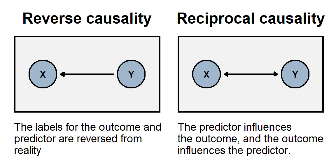
And (D) is similar, in the sense that racial bias might affect the length of sentence that was recommended by the district attorney.10.9 Reverse causality and reciprocal causality
The problem of reverse causality occurs when the association between our predictor and our outcome is because, in reality, the outcome causes variation in the predictor. In other words, we have the direction of causality backwards. For example, if we use the number of police officers per capita in a state to predict the homicide rate in a state, we might conclude that having more police officers causes a state to have a higher homicide rate. But the association might instead be because having a high homicide rates causes a state to hire more police officers.
The problem of reciprocal causality occurs when our predictor and our outcome affect each other. For example, imagine if reading the newspaper caused a person to have higher political knowledge, but having higher political knowledge increased how often a person read the newspaper. We could observe political knowledge associate with how often a person reads the newspaper, but we couldn’t use statistical control to validly estimate how much of that association is due to reading the newspaper.