8 Statistical control

8.1 Statistical control

Major learning objective(s) for this section:

Know how statistical control can help improve causal inference in non-experimental research.
For a given situation, propose and discuss a control variable that would be useful.
Correctly predict the effect of a particular control variable.

The nice thing about a randomized experiment is that the randomization means that there are only two possible reasons for a difference between groups in the experiment:

researchers treating the groups differently, and
random assignment error in which the groups were different before the researchers treated the groups differently.

Another nice thing about a randomized experiment is that a p-value under p=0.05 is sufficient in political science to consider random assignment error to not be a plausible explanation for the difference between groups. Therefore, if the p-value is p<0.05 for a difference between groups in randomized experiment, then in political science we can conclude that the difference in treatment plausibly caused the measured difference between groups.

But randomized experiments can’t be conducted for a lot of research questions. For example, we can’t randomly assign some countries to be democracies and randomly assign other countries to not be democracies. We can observe which countries are democracies and which countries are not democracies, but, on average, democracies differ from non-democracies in many ways other than the presence of democracy, such as GDP and education levels of their residents. Therefore, if we observe that democratic countries differ on average from non-democratic countries, we cannot reasonably conclude that such differences are because the countries have different levels of democracy, because the observed difference might have been caused by the difference between countries in GDP or the difference between countries in education levels of residents or the difference between countries in any other characteristic or combination of characteristics that differ between democracies and non-democracies.

However, researchers have tools that can help us make causal inferences even in the absence of the ability to conduct a randomized experiment. One such tool is called statistical control, in which researchers attempt to hold all else equal in a comparison, in order to isolate the effect of a single characteristic. The randomization of a randomized experiment can produce groups that are very similar to each other on all possible characteristics. The intent of statistical control is to make comparisons between subsets of groups that are similar to each other on all relevant characteristics, so that the comparison can isolate the effect of the factor that we are interested in.

The logic of statistical control is hold all else equal in comparisons between groups. Suppose, for instance, that a particular company paid male workers more on average than the company paid female workers on average. That gender gap could be due to the company’s unfair gender bias against female workers, but that gender gap could be due to other factors, such as if, on average, female workers chose to work fewer hours than male workers chose to work.

Let’s illustrate statistical control using the table below of hypothetical data for six workers at a company:

Gender	Pay	Time status	Gender	Pay	Time status
Male	$50	Full-time	Female	$50	Full-time
Male	$50	Full-time	Female	$20	Part-time
Male	$20	Part-time	Female	$20	Part-time

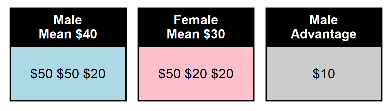
Based on the table, the mean pay is $40 among male workers and is $30 among female workers. So that’s a gender gap of $10 in mean pay per worker. Let’s first run an analysis that does not use statistical control:

Next, let’s control for full-time/part-time status, by comparing male workers to female workers at the same level of time status:

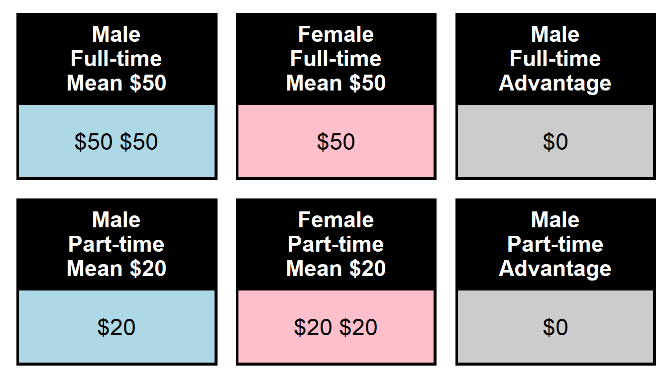
So when we compare the mean pay among male workers who work full-time to the mean pay among female workers who work full-time, there is no gap on average: both groups make $50 on average. And when we compare the mean pay among male workers who work part-time to the mean pay among female workers who work part-time, there is no gender gap: both groups make $20 on average. So – in the analysis without statistical control – the gender gap in pay favored men, but – when controlling for full-time/part-time status – there is no gender gap.

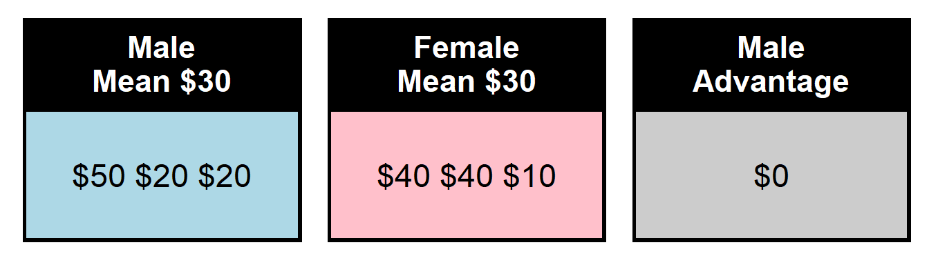
Statistical control can make an estimated difference smaller, make an estimated difference larger, or not change an estimated difference. Below is an example in which there is no gender gap in an analysis without statistical control – male workers make $30 on average, and female workers make $30 on average – but when controlling for time status – a gender gap appears, suggesting that female workers are unfairly paid less than male workers. Let’s start with the comparison without statistical control:

Gender	Pay	Time status	Gender	Pay	Time status
Male	$50	Full-time	Female	$40	Full-time
Male	$20	Part-time	Female	$40	Full-time
Male	$20	Part-time	Female	$10	Part-time

But below is the comparison with statistical control for time status:

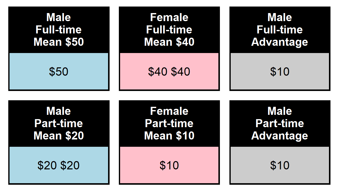
In a world without gender bias, worker pay would probably depend on more factors than whether a worker is full-time or part-time, and, thankfully, statistical control can involve more than one control variable. The logic is the same with more than one control variable. Suppose that we wanted to control for time status (full-time or part-time) and years of relevant work experience (from, say, 0 years of relevant work experience to 40 years of relevant work experience). For that analysis, we could compare the mean pay among full-time male workers with 0 years of relevant work experience to the mean pay among full-time female workers with 0 years of relevant work experience, then compare the mean pay among part-time male workers with 0 years of relevant work experience to the mean pay among part-time female workers with 0 years of relevant work experience, then compare the mean pay among full-time male workers with 1 year of relevant work experience to the mean pay among full-time female workers with 1 year of relevant work experience, and so on. Then we could average across each of these gaps to get an estimate of the overall gender gap in mean pay controlling for time status and years of relevant work experience.

Sample practice items

Statistical control helps causal inference in non-experimental research by…

eliminating measurement error in the outcome
getting groups similar to each other before the groups are treated differently
helping to address alternate explanations
adjusting the data to be normally distributed

Answer

helping to address alternate explanations

Suppose that you were asked to conduct a study to determine whether male ISU employees are paid more than female ISU employees are paid. For each ISU employee, you have data on the employee’s pay and their gender. Using these pay data as the outcome, would you need control variables for this study?

Answer

No
We are interested merely in whether male ISU employees are paid more than female ISU employees are paid, so there is no need to control for anything. However, if we were interested in whether male ISU employees are unfairly paid more or less than female ISU employees are paid, then we would need to control for alternate explanations such as hours worked.

Suppose that you were asked to conduct a study to determine whether male ISU employees are unfairly paid more than female ISU employees are paid. For each ISU employee, you have data on the employee’s pay and their gender. Using these pay data as the outcome, would you need control variables for this study?

Answer

Suppose that an analysis on data from a large representative set of college students indicated that college students who had majored in political science had a higher mean level of political knowledge at graduation than college students who had majored in earth science. The p-value for the difference in means was p<0.05. Is this sufficient evidence to conclude that, at least among the students in the study and at least on average, majoring in political science caused a higher mean level of political knowledge than majoring in earth science did?

Answer

Suppose that, for a POL 138 course, all students attend the first class meeting in person and take a pretest about content that will be taught during the course. The teacher then permits each student to choose whether the student will attend the remainder of the POL 138 class meetings in Zoom or in person, before the in-person POL 138 final exam. Half of the students choose the Zoom option, and half of the students choose the in-person option. A researcher is interested in the extent to which, compared to attending POL 138 in Zoom, attending POL 138 in person affected student scores on the final exam, at least on average. For this analysis, explain the benefit of controlling for the student’s score on the POL 138 pretest.

Answer

Controlling for the student’s score on the POL 138 pretest age helps address the alternate explanation that the difference between final exam scores for the “in person” students and final exam scores for the “Zoom” students was due to smarter students being more (or less) likely to choose the “in person” option.

Suppose that we conduct a study of all drunk driving convictions in Illinois from 2000 to 2015, and we discover that, on average, men convicted of drunk driving received longer sentences than women convicted of drunk driving. Propose control variables that should be included in an analysis to assess whether gender bias among judges causes men to be convicted of drunk driving to receive longer sentences than women convicted of drunk driving.

Answer

Good controls include but are not limited to:

property damage caused by the drivers
injuries and deaths caused by the drivers
driver blood alcohol content levels
number of prior DUIs

Below are data on the pay and experience of four male teachers and four female teachers:

Teacher	Gender	Pay	Years	Teacher	Gender	Pay	Years
1	Male	60	0	5	Female	60	0
				6	Female	60	0

2	Male	80	10	7	Female	80	10
3	Male	80	10	8	Female	80	10
4	Male	80	10

Calculate the gender gap in mean pay, between the mean pay of the four male teachers and the mean pay of the four female teachers.

Answer

Four male teachers: (60+80+80+80)/4 = 75
Four female teachers: (60+60+80+80)/4 = 70
Gender gap in mean pay is 5.

Below are data on the pay and experience of four male teachers and four female teachers:

Teacher	Gender	Pay	Years	Teacher	Gender	Pay	Years
1	Male	60	0	5	Female	60	0
				6	Female	60	0

2	Male	80	10	7	Female	80	10
3	Male	80	10	8	Female	80	10
4	Male	80	10

Compared to the gender gap in mean pay when not controlling for experience, indicate whether the gender gap in mean pay when controlling for experience would be larger, smaller, or the same size.

Answer

Smaller. The gender gap controlling foe experience should be zero, because experience completely explains pay: each teacher with high experience has a pay of 80, and each teacher with low experience has a pay of 60, so that the gender of the teacher does not seem to matter.

Below are data on the pay and experience of four male teachers and four female teachers:

Teacher	Gender	Pay	Years	Teacher	Gender	Pay	Years
1	Male	60	0	5	Female	60	0
2	Male	80	0
3	Male	80	0

4	Male	80	10	6	Female	80	10
				7	Female	80	10
				8	Female	80	10

Calculate the gender gap in mean pay, between the mean pay of the four male teachers and the mean pay of the four female teachers.

Answer

Four male teachers: (60+80+80+80)/4 = 75
Four female teachers: (60+80+80+80)/4 = 75
Gender gap in mean pay is 0.

Below are data on the pay and experience of four male teachers and four female teachers:

Teacher	Gender	Pay	Years	Teacher	Gender	Pay	Years
1	Male	60	0	5	Female	60	0
2	Male	80	0
3	Male	80	0

4	Male	80	10	6	Female	80	10
				7	Female	80	10
				8	Female	80	10

Compared to the gender gap in mean pay when not controlling for experience, explain whether the gender gap in mean pay when controlling for experience would be larger, smaller, or the same size.

Answer

Larger. The gender gap controlling for experience should NOT be zero, because experience does not completely explain pay: all teachers with high experience have a pay of 80, but – among teachers with low experience – female teachers make less (60) than men on average (60, 80, 80).

The table below contains information about six police officers.

Officer	Does the officer wear a body camera?	Officer age	Citizen complaints about the officer
1	Yes	20	20 complaints
2	Yes	40	5 complaints
3	Yes	40	5 complaints

4	No	20	30 complaints
5	No	20	30 complaints
6	No	40	15 complaints

The mean gap in citizen complaints is 15 complaints, between police officers who wore a body camera (10 complaints on average) and police officers who did not wear a body camera (25 complaints on average). Based on the table data, statistical control for the age of the police officer makes the body cameras seem ___ at reducing citizen complaints about an officer, compared to an analysis of the data without any statistical control.

less effective
as effective
more effective

Answer

less effective
Let’s compare younger officers:
Younger officer + Body camera = mean number of complaints of 20
Younger officer + No body camera = mean number of complaints of 30

Let’s compare older officers:
Older officer + Body camera = mean number of complaints of 5
Older officer + No body camera = mean number of complaints of 15

The younger officer gap is 10, and the older officer gap is 10, so the overall gap when controlling for age of the officer is 10 complaints on average. The pattern for this is that older officers get fewer complaints and older officers are more likely to wear a body camera, so that imbalance makes the body cameras look more effective at reducing complaints than the body cameras really are.

8.2 Multiple linear regression

Major learning objective(s) for this section:

Interpret coefficients and p-values from multiple linear regression output.

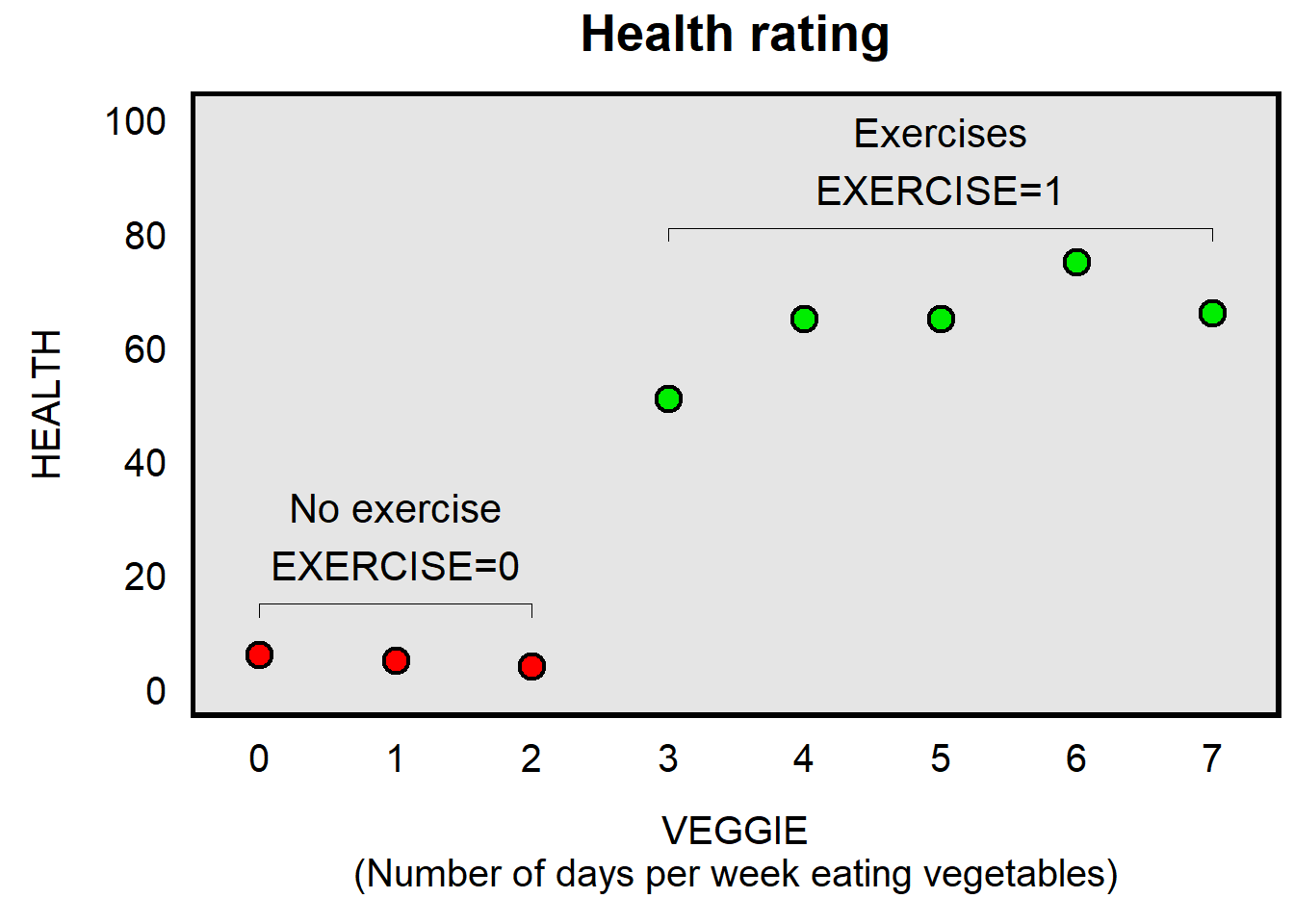
The plot below presents data for eight persons. The x-axis is VEGGIE, which indicates how many days per week that each of the eight persons eats vegetables, the y-axis is HEALTH, which indicates a rating about how healthy the person is, and the color of the dots indicates whether the person exercises, with a red dot indicating that the person does not exercise and a green dot indicating that the person exercises (with a variable called EXERCISE).

Let’s use linear regression to draw a line of best fit through these points, as shown below. The linear regression predicts the HEALTH rating using only the VEGGIE variable, so this plot colors all points black because this linear regression did not use data from the EXERCISE variable.

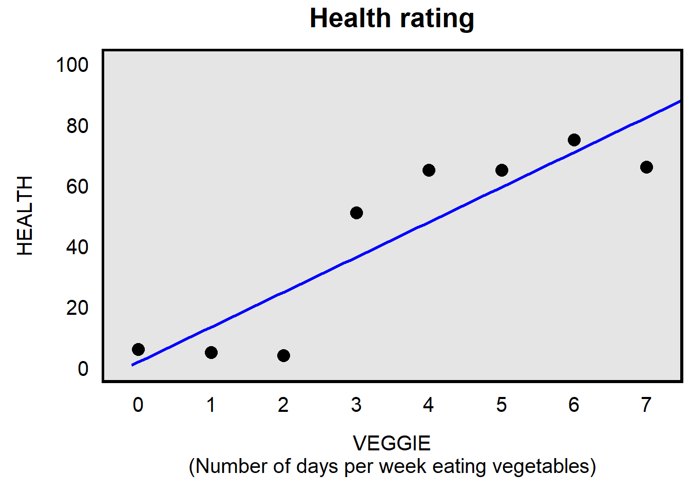
The output below is for the above linear regression. The intercept coefficient of 1.83 is the y-intercept, which indicates the predicted value of the outcome HEALTH when the predictor VEGGIE is set to zero. This can be interpreted as indicating that, based on the linear regression, a person who eats vegetables zero times per week would be predicted to have a HEALTH rating of 1.83. The coefficient of 11.51 for VEGGIE indicates the slope of the linear regression line. This can be interpreted as indicating that, compared to persons who eat vegetables a particular number of days per week, a person who eats vegetables one more day per week is predicted to have a HEALTH rating that is 11.51 units higher.

## MODEL INFO:
## Observations: 8
## Dependent Variable: HEALTH
## Type: OLS linear regression 
## 
## Standard errors:OLS
## ----------------------------------------------------------
##                      Est.     2.5%   97.5%   t val.      p
## ----------------- ------- -------- ------- -------- ------
## (Intercept)          1.83   -21.83   25.50     0.19   0.86
## VEGGIE              11.51     5.85   17.17     4.98   0.00
## ----------------------------------------------------------

Let’s use the linear regression output to write an equation for the line:

Y      =  b   +       mX
HEALTH = 1.83 + (11.38 * VEGGIE)

We can plug in values for VEGGIE to get a predicted HEALTH rating. For example, for a person who eats vegetables 4 times per week:

HEALTH = 1.83 + (11.51 * VEGGIE)
HEALTH = 1.83 + (11.51 * 4)      
HEALTH = 47.87

The line of best fit therefore runs through the point (X=4, Y=47.87).

In the above linear regression, the p-value for VEGGIE is p<0.05, so we can be confident at the conventional level in political science that, in these data, the association between VEGGIE and HEALTH is not due to random chance. But that doesn’t mean that we can conclude that eating vegetables more often caused people in the data to have a higher HEALTH rating. For all we know, people who eat vegetables more frequently are different in other important ways from people who eat vegetables less frequently, and these other differences might have caused part or all of the observed association between VEGGIE and HEALTH.

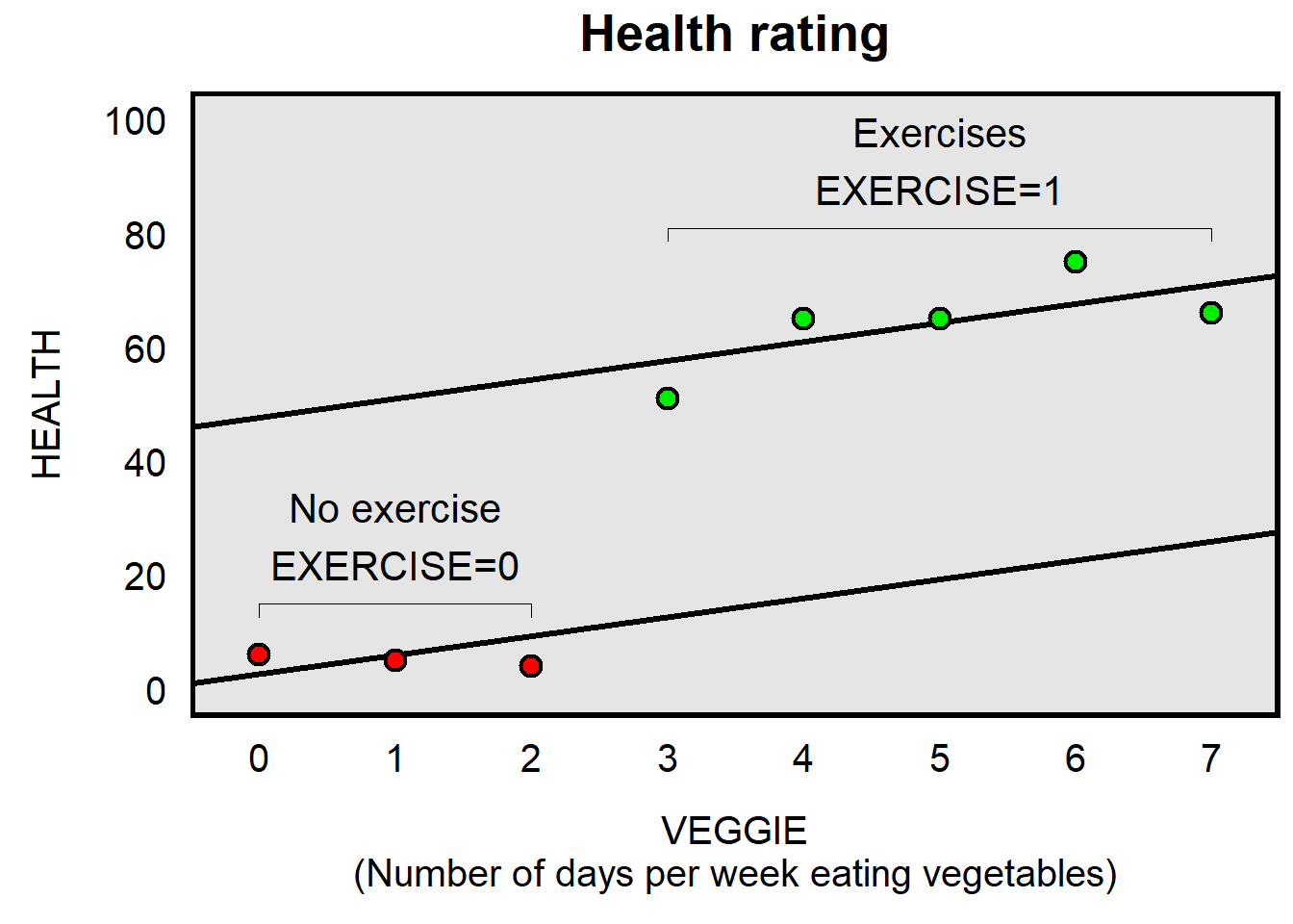
Let’s conduct another linear regression, but, this time, let’s control for whether a person exercises:

Below is the linear regression output:

## MODEL INFO:
## Observations: 8
## Dependent Variable: HEALTH
## Type: OLS linear regression 
## 
## Standard errors:OLS
## ---------------------------------------------------------
##                      Est.    2.5%   97.5%   t val.      p
## ----------------- ------- ------- ------- -------- ------
## (Intercept)          1.83   -8.04   11.70     0.48   0.65
## VEGGIE               3.17   -1.25    7.58     1.84   0.12
## EXERCISE            46.73   25.85   67.62     5.75   0.00
## ---------------------------------------------------------

The original coefficient on VEGGIE was 11.51. But, for the above linear regression with a control for EXERCISE, the coefficient on VEGGIE decreased to 3.17. This decrease is because much of the observed association between VEGGIE and HEALTH can be explained by the fact that people who eat vegetables more frequently also exercise, and this EXERCISE variable predicts the HEALTH rating better than the VEGGIE variable predicts the HEALTH rating.

In essence, in the regression in which the only predictor is VEGGIE, the VEGGIE coefficient is capturing the effect of VEGGIE and is capturing the effect of everything that is associated with VEGGIE, including EXERCISE. So, when EXERCISE is included in the regression as a control, the VEGGIE coefficient no longer captures the effect of EXERCISE. Of course, even with a control for EXERCISE, the VEGGIE coefficient might be capturing the effect of something else, so that we should be careful about interpreting the VEGGIE coefficient as indicating a causal effect. And, while, in this case, adding a control variable to the regression reduced the coefficient on the already-included predictor, it’s possible that adding a predictor increases the coefficient on the already-included predictor.

Let’s use this new linear regression output to write an equation for the line:

HEALTH = 1.83 + (3.17 * VEGGIE) + (46.73 * EXERCISE)

Like before, we can plug in values to get a prediction. Let’s get the predicted HEALTH rating for a person who eats vegetables 4 times per week and exercises:

HEALTH = 1.83 + (3.17 * VEGGIE) + (46.73 * EXERCISE)
HEALTH = 1.83 + (3.17 * 4)      + (46.73 * 1)
HEALTH = 61.24

Sample practice items

Let’s practice interpreting a linear regression, using survey data from the ANES 2016 Time Series Study. The output below predicts a participant’s ratings about Black Lives Matter (FTBLM) using predictors for the participant’s political party (PARTY06, coded from 0 for Strong Democrat to 6 for Strong Republican) and the participant’s race (coded as White, Black, Asian, or Other race):

## MODEL INFO:
## Observations: 3576 (694 missing obs. deleted)
## Dependent Variable: FTBLM
## Type: OLS linear regression 
## 
## Standard errors:OLS
## ----------------------------------------------------------
##                      Est.     2.5%   97.5%   t val.      p
## ----------------- ------- -------- ------- -------- ------
## (Intercept)         74.05    71.64   76.46    60.27   0.00
## PARTY06             -7.20    -7.62   -6.78   -33.76   0.00
## RACEWhite           -8.90   -11.34   -6.46    -7.16   0.00
## RACEBlack           13.75    10.14   17.35     7.48   0.00
## RACEAsian           -2.98    -8.33    2.37    -1.09   0.27
## ----------------------------------------------------------

The coefficient for PARTY06 in the linear regression output above indicates that, on average, ratings about Black Lives Matter are lower among Republicans than among Democrats, controlling for respondent race. Explain a benefit of the regression below controlling for race.

Answer

The control for respondent race addresses the alternate explanation that PARTY06 associates with FTBLM merely because of race. In the United States, Blacks are more likely to be Democrats than to be Republicans, so maybe the association between PARTY06 and FTBLM was merely because, compared to other people, Blacks are more likely to be Democrats and are more likely to highly rate Black Lives Matters. The regression controlling for race indicates that the association between PARTY06 and FTBLM holds on average across racial groups.

The linear regression below uses survey data from the ANES 2016 Time Series Study. The output below predicts a participant’s ratings about police (FTPOLICE) using predictors for the participant’s political party (PARTY06, coded from 0 for Strong Democrat to 6 for Strong Republican) and the participant’s race (coded as White, Black, Asian, or Other race):

## MODEL INFO:
## Observations: 3616 (654 missing obs. deleted)
## Dependent Variable: FTPOLICE
## Type: OLS linear regression 
## 
## Standard errors:OLS
## ----------------------------------------------------------
##                      Est.     2.5%   97.5%   t val.      p
## ----------------- ------- -------- ------- -------- ------
## (Intercept)         64.80    62.88   66.72    66.18   0.00
## PARTY06              2.37     2.03    2.70    13.89   0.00
## RACEWhite            6.74     4.80    8.69     6.79   0.00
## RACEBlack           -9.66   -12.53   -6.79    -6.60   0.00
## RACEAsian           -0.53    -4.78    3.71    -0.25   0.81
## ----------------------------------------------------------

Which of the following is the better interpretation of the 2.37 coefficient for PARTY06?

The predicted change in FTPOLICE for a one-unit increase in PARTY06.
The predicted change in FTPOLICE for a one-unit increase in PARTY06, controlling for respondent race.

Answer

The predicted change in FTPOLICE for a one-unit increase in PARTY06, controlling for respondent race.

8.3 Illustration of the effects of statistical control

The plots below are designed to illustrate that adding statistical control can change a coefficient that is already in a regression to be less extreme than the coefficient was before or to be more extreme than the coefficient was before.

Let’s start with the “less extreme” case. For this stylized example, we have three White respondents and three non-White respondents, with measures of respondent ratings about police (FTPOLICE) and respondent age (AGE) and the measure of race called WHITE coded as 1 for White and 0 for non-White. As indicated below, a control for participant race makes the AGE coefficient less extreme: the slope of the line of best fit for AGE is 0.48 in the left plot but is only 0.20 in the right plot.

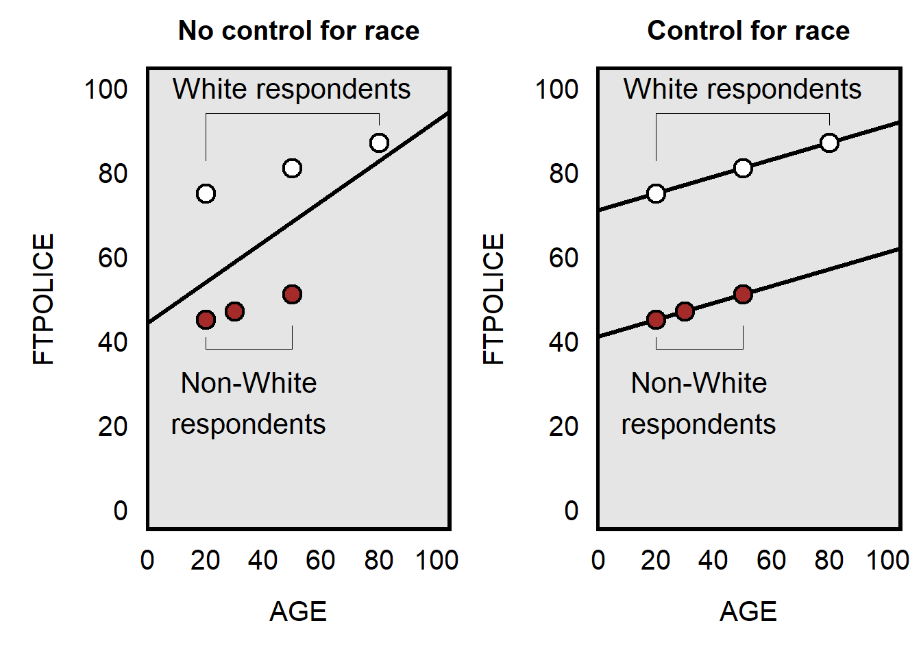
The mechanism in making the AGE coefficient less extreme is that, without a control for race, the AGE predictor is getting a boost from race: White respondents have more positive views of police, older respondents have more positive views of police, and older respondents are more likely to be White than to not be White. So the effect of age is mixed in with the effect of race. But controlling for race removes the effect of race from the coefficient for AGE.

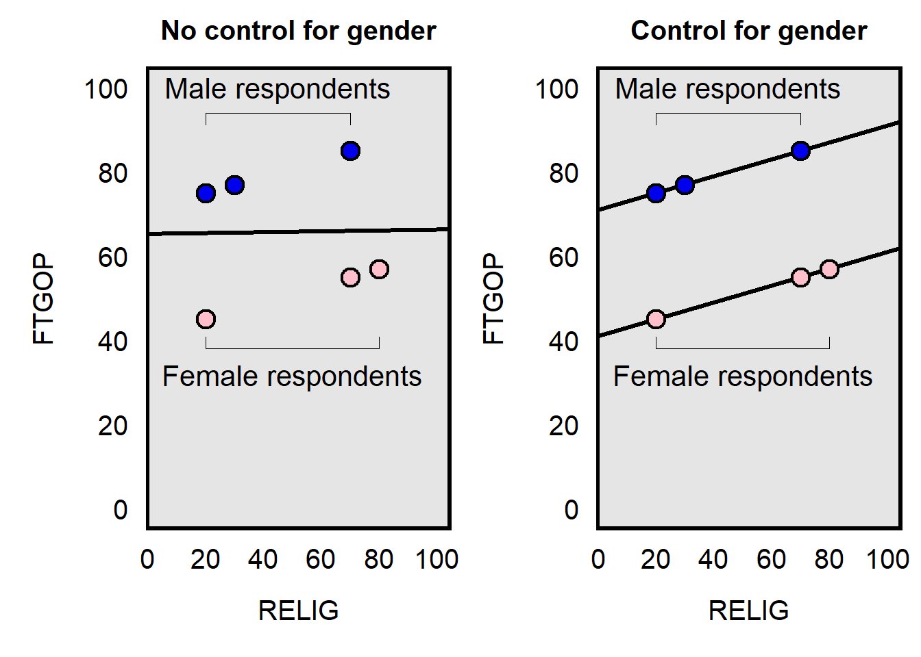
Let’s use a different stylized example to illustrate how adding statistical control can make a coefficient that is already in a regression be more extreme than the coefficient was before. For this example, we have three male respondents and three female respondents, with measures of respondent ratings about Republicans (FTGOP) and respondent religiosity (RELIG). As indicated below, a control for participant gender makes the coefficient for RELIG more extreme: the slope of the line of best fit for RELIG is 0.01 in the left plot but is 0.20 in the right plot.

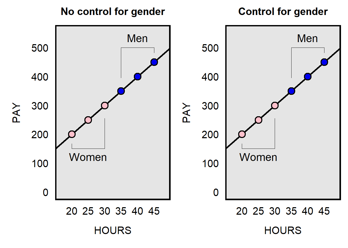
And to illustrate a situation in which statistical control does not affect the slope of a predictor already in the regression:

Sample practice items

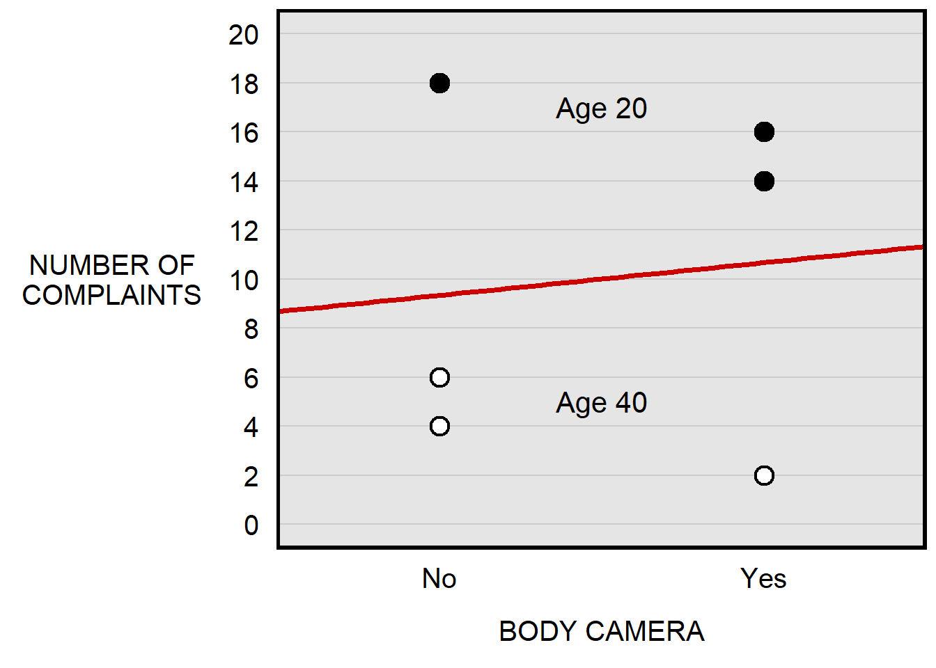
Each of the six dots in the plot below represents a police officer. The x-axis indicates whether the police officer wore a body camera this past year, and the y-axis indicates the number of complaints that citizens made against the police officer this past year. The black dots are for officers age 20, and the white dots are for officers age 40. The red line is the line of best fit through the points, indicating that police officers who wore a body camera received more complaints on average than police officers who did not wear a body camera; therefore, without any control variables, the plot suggests that the estimated effect of wearing a body camera is to increase the number of complaints that a police officer receives.

However, the plot also indicates that police officers who wore a body camera were on average younger than police officers who did not wear a body camera, which means that the effect of wearing a body camera is mixed in with the effect of the age of the officer. Based on the points, the estimated effect of wearing a body camera when controlling for the age of the police officer is to…

increase the number of complaints that the police officer receives
decrease the number of complaints that the police officer receives
not affect the number of complaints that the police officer receives

Answer

decrease the number of complaints that the police officer receives

Note that, within the age-20 police officers, the average number of complaints is 18 among police officers not wearing a body camera and is 15 among police officers wearing a body camera. Thus, among age-20 police officers, the estimated effect of wearing a body camera is to decrease complaints. And note that, within the age-40 police officers, the average number of complaints is 5 among police officers not wearing a body camera and is 2 among age-40 police officers wearing a body camera. Thus, among age-40 police officers, the estimated effect of wearing a body camera is to decrease complaints. Thus, overall, when controlling for the age of the police officer, the estimated effect of wearing a body camera is to decrease complaints.

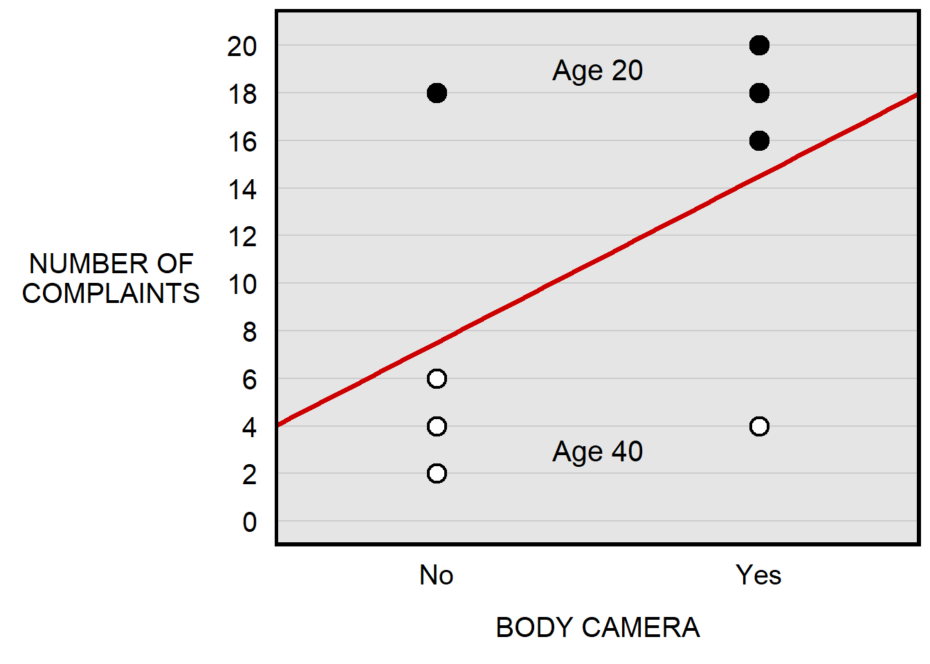
Each of the eight dots in the plot below represents a police officer. The x-axis indicates whether the police officer wore a body camera this past year, and the y-axis indicates the number of complaints that citizens made against the police officer this past year. The black dots are for officers age 20, and the white dots are for officers age 40. The red line is the line of best fit through the points, indicating that police officers who wore a body camera received more complaints on average than police officers who did not wear a body camera; therefore, without any control variables, the plot suggests that the estimated effect of wearing a body camera is to increase the number of complaints that a police officer receives.

increase the number of complaints that the police officer receives
decrease the number of complaints that the police officer receives
not affect the number of complaints that the police officer receives

Answer

not affect the number of complaints that the police officer receives

Note that, within the age-20 police officers, the average number of complaints is 18 among police officers not wearing a body camera and is also 18 among police officers wearing a body camera. Thus, among age-20 police officers, the estimated effect of wearing a body camera is zero. And note that, within the age-40 police officers, the average number of complaints is 4 among police officers not wearing a body camera and is also 4 among age-40 police officers wearing a body camera. Thus, among age-40 police officers, the estimated effect of wearing a body camera is zero. Thus, overall, when controlling for the age of the police officer, the estimated effect of wearing a body camera is zero.