18 Practice exam items
Practice for the Final Exam
The Final Exam is cumulative, with content drawn from Chapters 1 through 12, which were covered on Exams 1, 2, and 3.
Practice Final Exam (Word and PDF). Key available in docx and PDF
Practice for Exam 4
Exam 4 is a writing exam that covers Chapters 1 through 12.
Practice Exam 4 (Word and PDF). Key available in docx and PDF
Main eligible content for Exam 4:
Ability to explain why one research design is better than another research design
Ability to predict how a particular type of selection bias can bias an inference
Ability to propose an alternate explanation for a pattern
Ability to write the definition of a p-value, including all three key parts
Understanding of factors that can cause a null result that fails to detect a true effect
Understanding of how a difference-in-differences design can better help infer causality than a mere over-time difference can
Understanding of how comparison of cases just below and just above a threshold can help infer causality
Understanding of how statistical control can help infer causality
Understanding of how, for inferring causality, comparisons should try to hold constant as much as possible
Understanding of the benefit of weighting studies by sample size, for calculating an average effect size across studies
Understanding of the type of randomization that is needed for a randomized experiment and how that randomization can help identify the effect of a treatment
Understanding that a p-value of p<0.05 does not necessarily indicate a causal association
Practice for Exam 3
Exam 3 focuses on Chapter 9 through 12, but material from Chapters 1 through 8 is also eligible. The most missed items on Exam 2 were 41, 31, 10, 12, 38, 32, 19, 25, 40, and 34. Practice Exam 3 (Word and PDF). Key available in docx and PDF
See the sections below for more practice items for Chapters 9 through 12.
Practice for Exam 2
Exam 2 focuses on Chapter 5 through 8, but material from Chapters 1 through 4 is also eligible. The most missed items on Exam 1 were 29, 60, 28, 41, 45, 58, 61, 56, 30, and 59. Important concepts from Exam 1 include p-values and linear regression.
Practice Exam 2 (Word and PDF). Key available in docx and PDF
See the sections below for more practice items for Chapters 5 through 8.
Practice for Exam 1
Practice Exam 1 (Word and PDF) [Key]
1.1 Quantitative reasoning
Research focusing on numbers is…
- qualitative research
- quantitative research
Answer
- quantitative research
Which of these is closest to what an inference is?
- a conclusion
- a hypothesis
- a reason for a prediction
- a flawed idea
Answer
- a conclusion
1.2 Measures of central tendency
What is the mean of the set of numbers {0, 0, 1, 2, 7}?
- 0
- 1
- 2
- 10
- None of the above
Answer
- 2
What is the median of the set of numbers {0, 0, 1, 2, 7}?
- 0
- 1
- 2
- 10
- None of the above
Answer
- 1
What is the median of the set of numbers {0, 1, 3, 8}?
- 0
- 1
- 3
- 12
- None of the above
Answer
- None of the above
1.3 Outliers
Which number or numbers is or are an outlier in the set {-1, 0, 0, 1, 1001}?
- -1 only
- 0 only
- -1 and 1001 only
- 1001 only
- There is no outlier
Answer
- 1001 only
Adding an outlier to a set of data would be expected to have more influence on the ___ of the data.
- mean
- median
Answer
- mean
Removing an outlier from a set of data would be expected to have more influence on the ___ of the data.
- mean
- median
Answer
- mean
1.4 Standard deviation
Standard deviation is a measure of…
- central tendency
- correctness
- reliability
- validity
- variation
Answer
- variation
Which set of numbers – {1, 5} or {12, 14} – has a larger standard deviation?
- {1, 5}
- {12, 14}
- The standard deviations for the two sets would be the same.
Answer
- {1, 5}
Bob receives a 6 on each of his 4 exams. What is the standard deviation of Bob’s exam scores?
- 0
- 4
- 6
- 24
- None of the above
Answer
- 0
Bob recorded the temperatures in Celsius for the past few days, which were -2, -4, -5, and -1. What is known about the standard deviation of these temperatures?
- The standard deviation of these temperatures is less than zero.
- The standard deviation of these temperatures is zero.
- The standard deviation of these temperatures is greater than zero.
Answer
- The standard deviation of these temperatures is greater than zero.
Suppose that all students in a class take a 100-item test. The mean number of correct items on the test is 60, and the standard deviation of the number of correct items is 10. If the teacher counts each item correct as half of a point, the standard deviation of the test scores would be…
- lower than 10
- higher than 10
- 10
Answer
- lower than 10
Suppose that students in a class have weights of 80 kilograms, 90 kilograms, 100 kilograms, and 110 kilograms. The teacher multiplies each weight in kilograms by 2.2 to estimate the students’ weights in pounds. Compared to the students’ weights in kilograms, the students’ weights in pounds will have ___ number for the standard deviation.
- the same
- a lower
- a higher
Answer
- a higher
1.5 Histograms
In the histogram below, which is true?
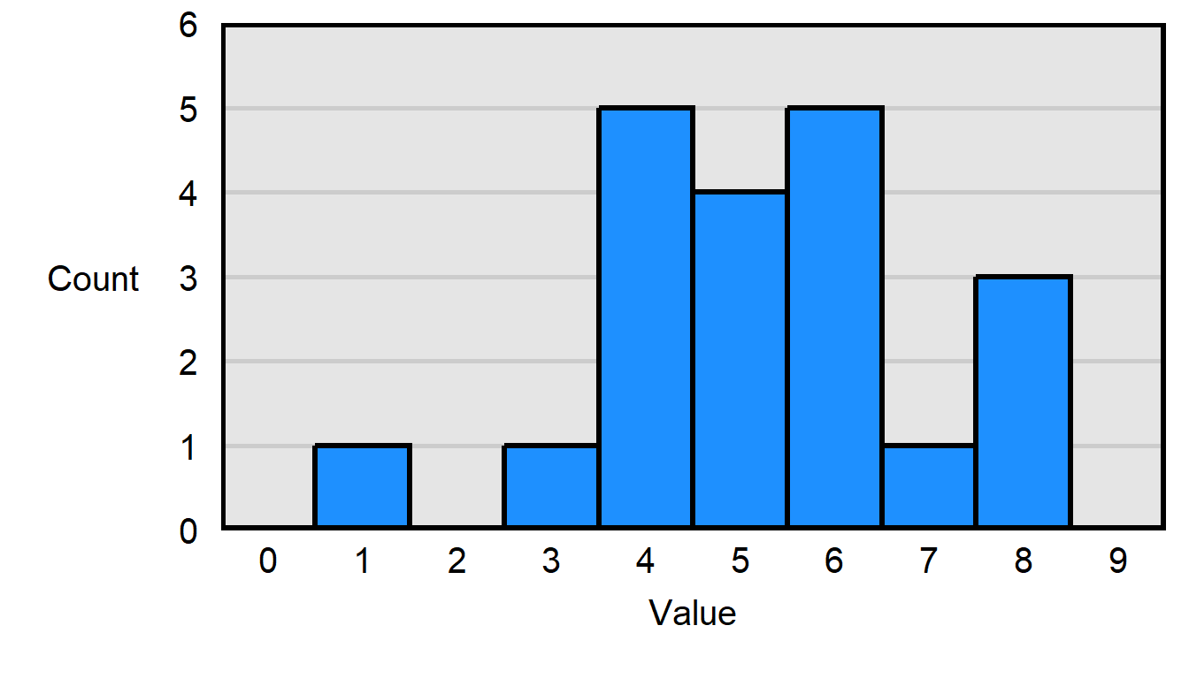
- There is 1 observation of 3.
- There are 3 observations of 1.
Answer
- There is 1 observation of 3.
1.6 Proportions, percentages, and percentage points
Suppose that a sample has 10 Democrats, 5 Independents, and 7 Republicans. What proportion of the sample is Independent, to two decimal places?
- 5 \(\div\) (10 + 7)
- 5 \(\div\) (10 + 5 + 7)
- (10 + 5 + 7) \(\div\) (10 + 5 + 7)
Answer
- 5 \(\div\) (10 + 5 + 7)
Suppose that, in 2023, 60% of students at a college are women, but that, in 2024, only 54% of students at the college are women. That change can be correctly expressed as a decrease of…
- 6 percent
- 6 percentage points
Answer
- 6 percentage points
Suppose that, in 2023, 60% of students at a college are women, but that, in 2024, only 54% of students at the college are women. That change can be correctly expressed as a decrease of…
- 10 percent
- 10 percentage points
Answer
- 10 percent
Suppose that, this year, 20% of students at a college are Republican, but that, next year, 40% of students at the college are Republican. That change can be correctly expressed as an increase of…
- 20 percent
- 20 percentage points
Answer
- 20 percentage points
Suppose that, this year, 20% of students at a college are Republican, but that, next year, 40% of students at the college are Republican. That change can be correctly expressed as an increase of…
- 100 percent
- 100 percentage points
Answer
- 100 percent
1.7 Percentiles
Suppose that a score of 70 is at the 80th percentile for scores on a test. What does this mean?
- 80 percent of scores are above 70.
- 80 percent of scores are below 70.
- 80 percent of scores were 70.
- A test with a score of 70 was a test with 80 percent of items correct.
- None of the above
Answer
- 80 percent of scores are below 70.
Suppose that the eight scores on a test are: 18, 34, 65, 75, 78, 81, 89, and 91. What percentile would the score of 89 be at, to the nearest whole percentile?
- 11th percentile
- 25th percentile
- 37th percentile
- 50th percentile
- 75th percentile
- 89th percentile
Answer
- 75th percentile
Which score below indicates a higher degree of political knowledge for a political knowledge test?
- scoring at the 1st percentile on the test
- scoring at the 99th percentile on the test
Answer
- scoring at the 99th percentile on the test
NBA basketball players tend to be taller than the average U.S. resident. Suppose that Bob is at the 80th percentile of height among U.S. residents. Bob’s percentile height among NBA basketball players is likely…
- less than the 80th percentile
- at the 80th percentile
- greater than the 80th percentile
Answer
- less than the 80th percentile
NBA basketball players tend to be taller than the average U.S. resident. Suppose that Bob is at the 80th percentile of height among NBA basketball players. Bob’s percentile height among U.S. residents is likely…
- less than the 80th percentile
- at the 80th percentile
- greater than the 80th percentile
Answer
- greater than the 80th percentile
1.8 Weighted means
Suppose that a course has three exams: Exam 1 is worth 10% of the overall grade for the course, Exam 2 is worth 30% of the overall grade for the course, and the Final Exam is worth 60% of the overall grade for the course. If a student scored 80% on Exam 1, 70% on Exam 2, and 90% on the Final Exam, what would be that student’s overall percentage for the course?
Answer
We can calculate the student’s final grade accounting for the fact that the final exam gets more weight than the midterm, by calculating the areas for each part of the final grade and them adding the areas together, as follows:
(0.10 \(\times\) 80) + (0.30 \(\times\) 70) + (0.60 \(\times\) 90) = 831.9 Probability
The probability of X happening is 40%, and the probability of Y happening is 20%. X and Y are independent events. What is the probability that X and Y both occur?
- 0.40 + 0.20
- 0.40 \(\times\) 0.20
- 0.40 \(\div\) 0.20
- (0.40 + 0.20) \(\div\) 2
- Cannot be determined from the information provided
Answer
- 0.40 \(\times\) 0.20
The probability of X happening is 40%, and the probability of Y happening is 20%. X and Y are not independent events. What is the probability that X and Y both occur?
- 0.40 + 0.20
- 0.40 \(\times\) 0.20
- 0.40 \(\div\) 0.20
- (0.40 + 0.20) \(\div\) 2
- Cannot be determined from the information provided
Answer
- Cannot be determined from the information provided
The probability of getting heads on each flip of a fair coin is 50%, and one flip of the coin does not influence another flip of the coin. Using the product rule, what is the probability of flipping a fair coin twice and getting two heads?
- 0.50 + 0.50
- 0.50 \(\times\) 0.50
- The product rule should not be used for this item.
Answer
- 0.50 \(\times\) 0.50
Suppose that you flip a fair coin one thousand times. Is it possible that all of the flips land on heads?
- Yes
- No
Answer
- Yes
This reflects a problem with making inferences about the fairness of a coin based merely on flipping the coin: any outcome that we observe with a coin (such as 1,000 heads in 1,000 flips) could have occurred with a fair coin.
Suppose that, in a given population, 40% of persons are men and 40% of persons are Republicans. Suppose that we want to calculate the probability that a given person randomly selected from this population is a Republican man. Can we use the product rule to calculate that probability as being \(0.40\times0.38\), to get a 16% probability that that randomly selected person is a Republican man?
Answer
The product rule cannot be used in this situation because the probability of being a man might not be independent of the probability of being a Republican. For example, in the United States, men are currently more likely than woman to identify as Republican than as a Democrat.Suppose that the Freedonia Senate has 70 men senators and 30 women senators. Three senators are randomly selected to be on the Education Committee. Which one of the following indicates the probability that all four senators are men?
- (70 \(\div\) 100) \(\times\) 3
- (70 \(\div\) 100) \(\times\) (30 \(\div\) 100)
- (70 \(\div\) 100)3
- (70 \(\div\) 100) \(\times\) (69 \(\div\) 99) \(\times\) (68 \(\div\) 98)
- (70 \(\div\) 100) \(\times\) (69 \(\div\) 100) \(\times\) (68 \(\div\) 100)
Answer
The probability that the first senator is a man is (70 \(\div\) 100). But once a man has been selected for the Education Committee, that man cannot be selected again, so that there is one fewer man to select and one fewer senator that can be selected.2.1 Sampling error
Suppose that a researcher is interested in estimating the percentage of students at U.S. universities who voted in the 2022 midterm elections, so the researcher samples 400 students at Illinois State University.
The researcher’s population is best described as…
- students at U.S. universities
- the 400 students at Illinois State University
Answer
- students at U.S. universities
Suppose that a researcher is interested in estimating the percentage of students at U.S. universities who voted in the 2022 midterm elections, so the researcher samples 400 students at Illinois State University.
The researcher’s sample is best described as…
- students at U.S. universities
- the 400 students at Illinois State University
Answer
- the 400 students at Illinois State University
2.2 Law of Large Numbers
Amy and Bob are estimating the mean political ideology of students at Illinois State University. Amy emails all 3,800 business majors at ISU, asks them to rate their political ideology on a scale from 0 for very liberal to 100 for very conservative, and then calculates the mean political ideology among these students; each of these 3,800 business majors responded to Amy’s email. Bob randomly emails 600 ISU students, asks them to rate their political ideology on a scale from 0 for very liberal to 100 for very conservative, and then calculates the mean political ideology among these students; each of these 600 students responded to Bob’s email. Who has a more credible estimate of the mean political ideology of ISU students?
- Amy, because her sample size is larger
- Amy, because her sample included all business majors
- Bob, because his sample size is smaller
- Bob, because he used a random sample of the population
Answer
- Bob, because he used a random sample of the population
Amy flips a fair coin 20 times. Bob flips a fair coin 300 times. Compared to the percentage heads among Amy’s coin flips, the percentage heads among Bob’s coin flips is expected to be…
- lower
- higher
- closer to 50%
- farther from 50%
Answer
- closer to 50%
Suppose that a population is 40% male. Which sample below is more likely to be closer to 40% male?
- a random sample of 40 members of the population
- a random sample of 120 members of the population
Answer
- a random sample of 120 members of the population
Suppose that a school randomly assigns students to a small class of 10 students or to a large class of 50 students, so that 20 classes in the school are small classes and 20 classes in the school are large classes. The school calculates the mean weight of students for each of these 40 classes, so that each class has one mean weight and there are a total of 40 mean class weights.
Across these 40 mean class weights, which would be most likely about the class that has the lowest mean class weight?
- It is likely to be a small class.
- It is likely to be a large class.
- It is just as likely to be a small class as a large class.
Answer
- It is likely to be a small class.
Suppose that a school randomly assigns students to a small class of 10 students or to a large class of 50 students, so that 20 classes in the school are small classes and 20 classes in the school are large classes. The school calculates the mean weight of students for each of these 40 classes, so that each class has one mean weight and there are a total of 40 mean class weights.
Across these 40 mean class weights, which would be most likely about the class that has the highest mean class weight?
- It is likely to be a small class.
- It is likely to be a large class.
- It is just as likely to be a small class as a large class.
Answer
- It is likely to be a small class.
Amy randomly samples 80 ISU students and asks them to rate the U.S. president on a scale from 0 for very cold to 100 for very warm. Bob randomly samples 250 ISU students and asks them to rate the U.S. president on a scale from 0 for very cold to 100 for very warm. Which of the following, if any, should be expected due to this difference in sample size?
- The mean support for the president is likely to be lower in Amy’s sample than in Bob’s sample.
- The mean support for the president is likely to be higher in Amy’s sample than in Bob’s sample.
- Neither of the above
Answer
- Neither of the above
2.3 Imbalanced sample sizes
Suppose that we want to test the null hypothesis that the percentage of Illinois Democrats who support lowering the voting age to 12 equals the percentage of Illinois Republicans who support lowering the voting age to 12. Which set of samples below would be better for testing this null hypothesis?
- a random sample of 300 Illinois Democrats and a random sample of 300 Illinois Republicans
- a random sample of 400 Illinois Democrats and a random sample of 600 Illinois Republicans
Answer
- a random sample of 400 Illinois Democrats and a random sample of 600 Illinois Republicans
Amy randomly samples 30 ISU students and asks them to rate the president on a scale from 0 for very cold to 100 for very warm. Bob randomly samples 200 ISU students and asks them to rate the president on a scale from 0 for very cold to 100 for very warm. Which of the following, if any, should be expected due to this difference in sample size?
- The mean support for the president is likely to be lower in Amy’s sample than in Bob’s sample.
- The mean support for the president is likely to be higher in Amy’s sample than in Bob’s sample.
- Neither of the above
Answer
- Neither of the above
2.5 Sampling weights
Political scientists weight survey data for which of the following reasons?
- Because the sample is too small
- Because the population is much larger than the sample
- Because the sample characteristics do not match the population characteristics
Answer
- Because the sample characteristics do not match the population characteristics
Suppose that men are 70% of a population and women are 30% of the population. Men are 50% of our sample of the population, and women are 50% of our sample of the population. Men in our sample had a mean height of 180cm, and women in our sample had a mean height of 170cm. What would be the best estimate for the mean height of the population, assuming that the samples are representative?
- (0.70 \(\times\) 170cm) + (0.30 \(\times\) 180cm) = 173cm
- (0.50 \(\times\) 180cm) + (0.50 \(\times\) 170cm) = 175cm
- (0.70 \(\times\) 180cm) + (0.30 \(\times\) 170cm) = 177cm
Answer
We are estimating the population mean height, so we can ignore the sample percentages. The problem then becomes a weighted mean problem, so:
- (0.70 \(\times\) 180cm) + (0.30 \(\times\) 170cm) = 177cm
If Asians are 10 percent of a sample and 6 percent of a population, what weight should be applied to each Asian person in the sample, if weighting on only race?
- 6 + 10
- 6 \(\div\) 10
- 10 + 6
- 10 \(\div\) 6
- None of the above
Answer
- 6 \(\div\) 10 The survey weight formula in general is population divided by sample, so, for this item, the survey weight for Asians is 6 \(\div\) 10.
If the mean survey weight for a group is 0.4, then that means that the group was…
- undersampled, relative to the group’s percentage of the population
- oversampled, relative to the group’s percentage of the population
- neither undersampled nor oversampled, relative to the group’s percentage of the population
Answer
- oversampled, relative to the group’s percentage of the population
If the mean survey weight for a group is 1, then that means that the group was…
- undersampled, relative to the group’s percentage of the population
- oversampled, relative to the group’s percentage of the population
- neither undersampled nor oversampled, relative to the group’s percentage of the population
Answer
- neither undersampled nor oversampled, relative to the group’s percentage of the population
If the mean survey weight for a group is 1.3, then that means that the group was…
- undersampled, relative to the group’s percentage of the population
- oversampled, relative to the group’s percentage of the population
- neither undersampled nor oversampled, relative to the group’s percentage of the population
Answer
- undersampled, relative to the group’s percentage of the population
2.6 The normal distribution
The image below is an example of a…
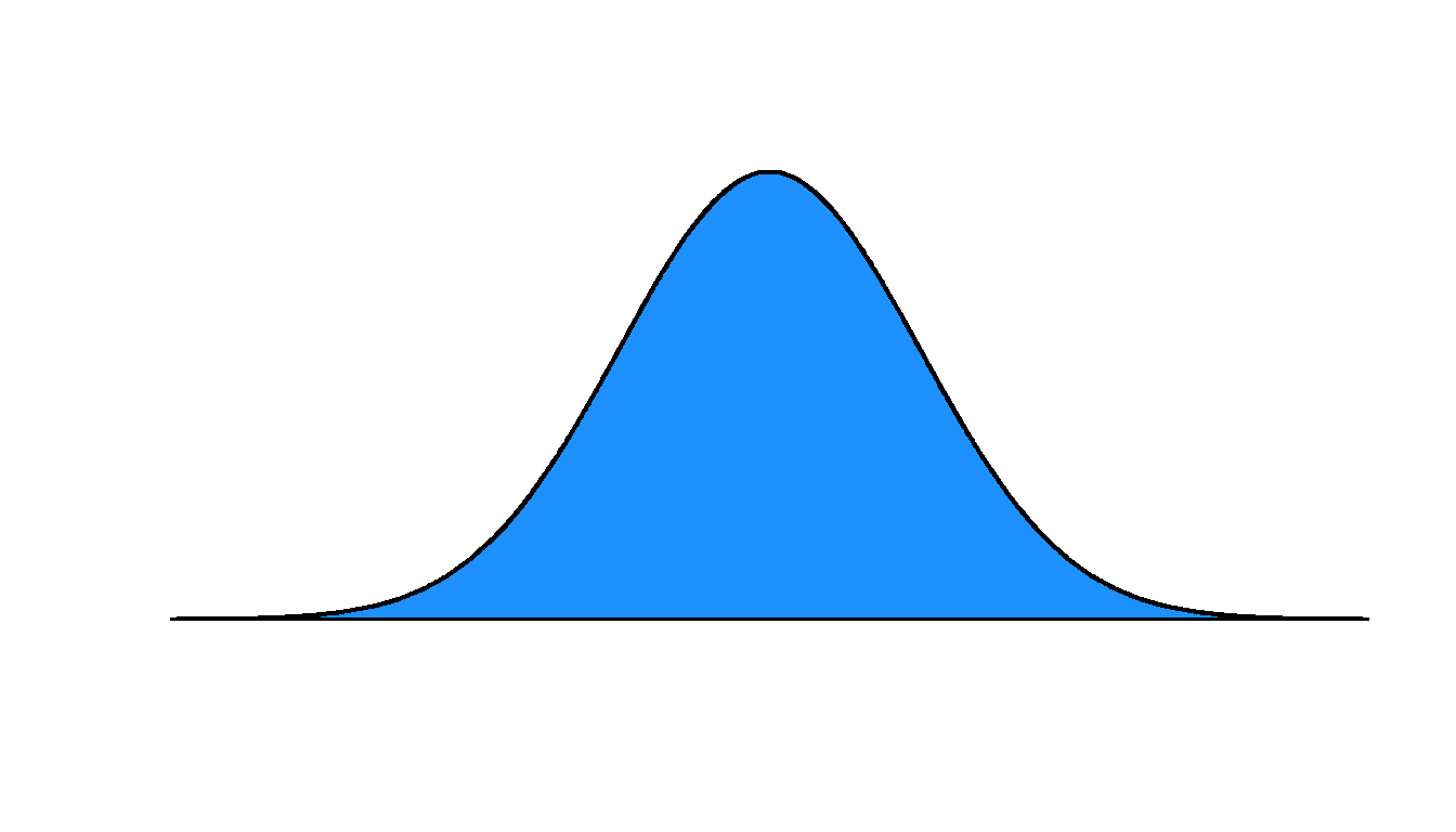
- uniform distribution
- normal distribution
Answer
- normal distribution
The image below is an example of a…
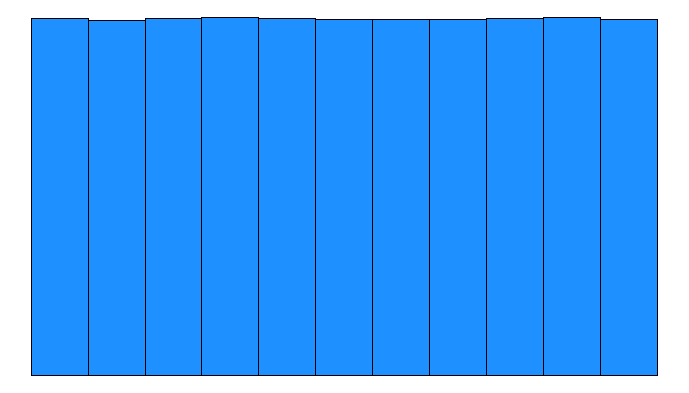
- uniform distribution
- normal distribution
Answer
- uniform distribution
Suppose that, in a set of 101 adults, each whole number weight from 150 lbs to 250 lbs appears exactly once (e.g., 150, 151, 152, …, 249, 250). We randomly select ten of these adults and plot the mean weight of this sample of ten adults. We randomly select another ten of these adults (which might include some adults already selected) and plot the mean weight of this second sample of ten adults. We continue until we plot 2,000 means. A histogram of the means is expected to be…
- uniform distribution
- non-uniform distribution
Answer
- non-uniform distribution
Suppose that we have a set of the ten whole numbers from 0 to 9, of {0,1,2,3,4,5,6,7,8,9}. We randomly select a number from this set and then add that number to a brand new empty database. We randomly select another number from this set (which might or might not have already been selected) and then add that number to the same database, so that the database now has two numbers. We do this over and over again until the database has 40,000 numbers. A histogram of the numbers in the database is expected to be…
- uniform distribution
- non-uniform distribution
Answer
- uniform distribution
Suppose that a test has a mean of 100 and a standard deviation of 10. Scores on the test follow a normal distribution. About 95% of scores should fall within which two scores?
- 90 and 110, which is ± 1 standard deviation
- 80 and 120, which is ± 2 standard deviations
- 70 and 130, which is ± 3 standard deviations
- 60 and 120, which is ± 4 standard deviations
- 10 and 100, which is ± 5 standard deviations
Answer
- 80 and 120, which is ± 2 standard deviations
The 600 scores in Group A follow a normal distribution and have a mean of 100 and a standard deviation of 5. The 600 scores in Group B follow a normal distribution and have a mean of 100 and a standard deviation of 20. Based on these statements, which one of the following statements is true?
- It is more likely that Group A has the highest score, and not Group B.
- It is more likely that Group B has the highest score, and not Group A.
- The probability that Group A has the highest score is the same as the probability that Group B has the highest score.
Answer
- It is more likely that Group B has the highest score, and not Group A.
The 600 scores in Group A follow a normal distribution and have a mean of 100 and a standard deviation of 5. The 600 scores in Group B follow a normal distribution and have a mean of 100 and a standard deviation of 20. Based on these statements, which one of the following statements is true?
- It is more likely that Group A has the lowest score, and not Group B.
- It is more likely that Group B has the lowest score, and not Group A.
- The probability that Group A has the lowest score is the same as the probability that Group B has the lowest score.
Answer
- It is more likely that Group B has the lowest score, and not Group A.
Suppose that scores on a national test follow a normal distribution and have a mean of 100 and a standard deviation of 10. If Student A raises her score from 90 to 100, and Student B raises her score from 120 to 130, which of the following statements is true?
- Student A had the higher percentile increase on the test.
- Student B had the higher percentile increase on the test.
- Student A had the same percentile increase on the test as Student B had.
Answer
- Student A had the higher percentile increase on the test.
Suppose that scores on a national test follow a normal distribution and have a mean of 100 and a standard deviation of 10. If Student A raises her score from 90 to 100, and Student B raises her score from 100 to 110, which of the following statements is true?
- Student A had the higher percentile increase on the test.
- Student B had the higher percentile increase on the test.
- Student A had the same percentile increase on the test as Student B had.
Answer
- Student A had the same percentile increase on the test as Student B had.
2.7 Confidence intervals
Which of the following is expected to be wider?
- the 95% confidence interval for the mean weight of a random sample of 10 U.S. residents
- the 95% confidence interval for the mean weight of a random sample of 200 U.S. residents
Answer
- the 95% confidence interval for the mean weight of a random sample of 10 U.S. residents
For a given estimate, all else equal, which of the following would be the wider?
- 90% confidence interval
- 99% confidence interval
Answer
- 99% confidence interval
Amy randomly samples 30 ISU students and asks them to rate the president on a scale from 0 for very cold to 100 for very warm. Bob randomly samples 200 ISU students and asks them to rate the president on a scale from 0 for very cold to 100 for very warm. Which of the following, if any, should be expected due to this difference in sample size?
- The 95% confidence interval for mean support for the president is thinner in Amy’s sample than in Bob’s sample.
- The 95% confidence interval for mean support for the president is wider in Amy’s sample than in Bob’s sample.
- Neither of the above
Answer
- The 95% confidence interval for mean support for the president is wider in Amy’s sample than in Bob’s sample.
3.1 The null hypothesis
Which best indicates what the null hypothesis is?
- The hypothesis being tested
- The hypothesis that is true
- The hypothesis that the effect is not zero
- The hypothesis that is most supported by the evidence
Answer
- The hypothesis being tested
Suppose that the null hypothesis is that a treatment will have a negative effect. Which of the following would be the alternate hypothesis?
- The treatment will have no effect.
- The treatment will have a positive effect.
- The treatment will not have a negative effect.
Answer
- The treatment will not have a negative effect.
3.2 p-values
Of the following, which best describes what a p-value measures?
- the precision of an estimate
- the strength of evidence against the null hypothesis
- the size of an association controlling for other model factors
Answer
- the strength of evidence against the null hypothesis
Of the p-values below, which p-value is the strongest evidence that an observed difference between the percentage of heads and the percentage of tails from a set of coin flips would have been unlikely to have occurred due to random chance, if the coin is fair?
- 0.01
- 0.05
- 0.99
- 1.00
Answer
- 0.01
If we flipped a coin 12 times and got 6 heads and 6 tails, what would be the p-value for a statistical test of the null hypothesis that the coin is fair?
- 0
- 1
- something between 0 and 1
Answer
- 1
A p-value is a measure of the strength of the evidence that an analysis has provided against the null hypothesis. If an analysis has provided no evidence against the null hypothesis, the p-value is 1.
In this case, there is no evidence against the null hypothesis that the coin is fair.If we flipped a coin 12 times and got 2 heads and 10 tails, what would be the p-value for a statistical test of the null hypothesis that the coin is fair?
- 0
- 1
- something between 0 and 1
Answer
- something between 0 and 1
A p-value is a measure of the strength of the evidence that an analysis has provided against the null hypothesis. If an analysis has provided no evidence against the null hypothesis, the p-value is 1. The lower the p-value, the more evidence the analysis has provided against the null hypothesis. A p-value of zero would indicate that the analysis has provided infinitely strong evidence against the null hypothesis.
In this case, there is some evidence against the null hypothesis that the coin is fair.If we flipped a coin 12 times and got 0 heads and 12 tails, what would be the p-value for a statistical test of the null hypothesis that the coin is fair?
- 0
- 1
- something between 0 and 1
Answer
- something between 0 and 1
A p-value is a measure of the strength of the evidence that an analysis has provided against the null hypothesis. If an analysis has provided no evidence against the null hypothesis, the p-value is 1. The lower the p-value, the more evidence the analysis has provided against the null hypothesis. A p-value of zero would indicate that the analysis has provided infinitely strong evidence against the null hypothesis.
In this case, there is some evidence against the null hypothesis that the coin is fair.Suppose that, in an experiment, the mean for the control group was 2, the standard deviation for the control group was 2, the mean for the treatment group was 2, and the standard deviation for the treatment group was 3. What would be the p-value for a test of the null hypothesis that the control group mean equals the treatment group mean?
- 0
- 1
- something between 0 and 1
Answer
- 1
A p-value is a measure of the strength of the evidence that an analysis has provided against the null hypothesis. If an analysis has provided no evidence against the null hypothesis, the p-value is 1.
In this case, there is no evidence against the null hypothesis that the control group mean equals the treatment group mean.Suppose that, in an experiment, the mean for the control group was 4, the standard deviation for the control group was 3, the mean for the treatment group was 2, and the standard deviation for the treatment group was 1. What would be the p-value for a test of the null hypothesis that the control group mean equals the treatment group mean?
- 0
- 1
- something between 0 and 1
Answer
- something between 0 and 1
A p-value is a measure of the strength of the evidence that an analysis has provided against the null hypothesis. If an analysis has provided no evidence against the null hypothesis, the p-value is 1. The lower the p-value, the more evidence the analysis has provided against the null hypothesis. A p-value of zero would indicate that the analysis has provided infinitely strong evidence against the null hypothesis.
In this case, there is some evidence against the null hypothesis that the control group mean equals the treatment group mean.3.3 Estimating p-values
The histogram below is from a simulation that had a large number of flips of a fair coin. The horizontal x-axis indicates each number of times that the fair coin could land on heads in the six flips, and the height of the columns indicates the number of times the fair coin landed on that number of heads in the six flips. For example, the 9.4% for the x-axis value of 5 indicates that the fair coin landed on heads exactly 5 times in the 6 flips in 9.4% of the 100,000 trials.
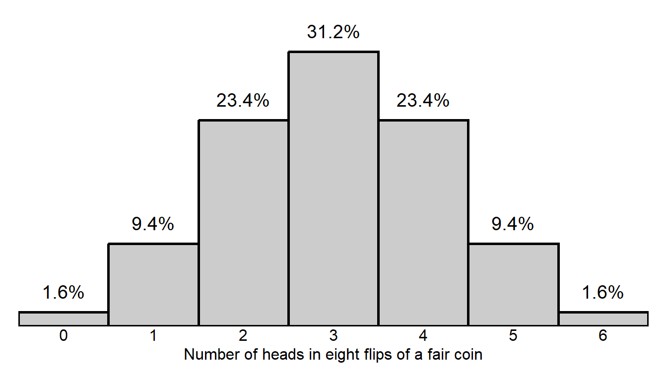
Based on the above simulation data, which of the following calculations indicates the p-value that would occur for a test of the null hypothesis that a coin is fair, if the coin landed on 5 heads in 6 flips? Note that percentages in the options are expressed as decimals, so, for example, 9.4% is 0.094.
- 0.094
- 0.094 + 0.016
- 0.013 + 0.094 + 0.094 + 0.016
- 0.094 + 0.234 + 0.312 + 0.234 + 0.094
Answer
- 0.013 + 0.094 + 0.094 + 0.016
3.4 p-values if the null hypothesis is true
Suppose that we conduct 900 well-designed independent tests of a null hypothesis. In reality, the null hypothesis is true. What is the expected percentage of these tests that are expected to have a p-value of p<0.05?
- 0%
- 5%
- 50%
- 95%
- 100%
- Cannot be determined without more information
Answer
- 5%
3.5 p-values if the null hypothesis is not true
In the original setup for an experiment, the outcome variable is coded from 0 through 20, the mean of the outcome variable is 8 for Group A and is 11 for Group B, the standard deviation of the outcome variable is 9 for Group A and is 9 for Group B, and the sample size is 100 for Group A and is 100 for Group B. The p-value is p=0.02 for a test of the null hypothesis that the mean of the outcome variable for Group A equals the mean of the outcome variable for Group B.
Suppose that everything else were the same as in the original setup, but the sample sizes were 200 for Group A and 200 for Group B. Which of the following, if any, would we know about the p-value for a test of the null hypothesis that the mean of the outcome variable for Group A equals the mean of that outcome variable for Group B?
- The p-value would be p=0.02
- The p-value would be less than p=0.02
- The p-value would be greater than p=0.02
Answer
- The p-value would be less than p=0.02
In the original setup for an experiment, the outcome variable is coded from 0 through 20, the mean of the outcome variable is 8 for Group A and is 11 for Group B, the standard deviation of the outcome variable is 9 for Group A and is 9 for Group B, and the sample size is 100 for Group A and is 100 for Group B. The p-value is p=0.02 for a test of the null hypothesis that the mean of the outcome variable for Group A equals the mean of the outcome variable for Group B.
Suppose that everything else were the same as in the original setup, but the standard deviation of responses were 6 for Group A and 6 for Group B. Which of the following, if any, would we know about the p-value for a test of the null hypothesis that the mean of the outcome variable for Group A equals the mean of that outcome variable for Group B?
- The p-value would be p=0.02
- The p-value would be less than p=0.02
- The p-value would be greater than p=0.02
Answer
- The p-value would be less than p=0.02
In the original setup for an experiment, the outcome variable is coded from 0 through 20, the mean of the outcome variable is 8 for Group A and is 11 for Group B, the standard deviation of the outcome variable is 9 for Group A and is 9 for Group B, and the sample size is 100 for Group A and is 100 for Group B. The p-value is p=0.02 for a test of the null hypothesis that the mean of the outcome variable for Group A equals the mean of the outcome variable for Group B.
Suppose that everything else were the same as in the original setup, but the mean response was 8 for Group A and 14 for Group B. Which of the following, if any, would we know about the p-value for a test of the null hypothesis that the mean of the outcome variable for Group A equals the mean of that outcome variable for Group B?
- The p-value would be p=0.02
- The p-value would be less than p=0.02
- The p-value would be greater than p=0.02
Answer
- The p-value would be less than p=0.02
In the original setup for an experiment, the outcome variable is coded from 0 through 20, the mean of the outcome variable is 8 for Group A and is 11 for Group B, the standard deviation of the outcome variable is 9 for Group A and is 9 for Group B, and the sample size is 100 for Group A and is 100 for Group B. The p-value is p=0.02 for a test of the null hypothesis that the mean of the outcome variable for Group A equals the mean of the outcome variable for Group B.
Suppose that everything else were the same as in the original setup, but the standard deviation of responses were 12 for Group A and 12 for Group B. Which of the following, if any, would we know about the p-value for a test of the null hypothesis that the mean of the outcome variable for Group A equals the mean of that outcome variable for Group B?
- The p-value would be p=0.02
- The p-value would be less than p=0.02
- The p-value would be greater than p=0.02
Answer
- The p-value would be greater than p=0.02
3.6 Hypothesis testing
What is the conventional p-value threshold in political science?
- 0
- 0.01
- 0.05
- 0.50
- 0.95
- 0.99
- 1
Answer
- 0.05
If the p-value for a test of a null hypothesis is p=0.02, then we should do which of the following?
- accept the null hypothesis and accept the alternative hypothesis
- reject the null hypothesis and reject the alternative hypothesis
- accept the null hypothesis and reject the alternative hypothesis
- reject the null hypothesis and accept the alternative hypothesis
- none of the above
Answer
- reject the null hypothesis and accept the alternative hypothesis
A researcher tested the null hypothesis that an association is zero. The p-value for this test p=0.91. Based on this p-value, which of the following should the researcher do, using the conventional level in political science?
- conclude that the association is zero
- conclude that the association is not zero
- neither of the above
Answer
- neither of the above
A researcher tested the null hypothesis that an association is zero. The p-value for this test p<0.05. Based on this p-value, which of the following should the researcher do, using the conventional level in political science?
- conclude that the association is zero
- conclude that the association is not zero
- neither of the above
Answer
- conclude that the association is not zero
A researcher tested the null hypothesis that an association is zero. The p-value for this test p=0.30. Based on this p-value, which of the following should the researcher do, using the conventional level in political science?
- conclude that the association is zero
- conclude that the association is not zero
- neither of the above
Answer
- neither of the above
3.7 Selecting a p-value threshold
Suppose that we are testing patient blood samples for evidence of the presence of a new virus. If there is sufficient evidence in the blood sample for the presence of the new virus, we will prescribe the patient a pill that has no negative effects and that can help combat the new virus. Our null hypothesis is that the blood sample does not have the new virus. Which p-value threshold below would be more appropriate, if we prefer to avoid not prescribing the pill to patients whose blood contains the new virus?
- p=0.01
- p=0.10
Answer
- p=0.10
Suppose that we are testing for gender bias among ISU students in student evaluations of teachers. Our null hypothesis is that there is no gender bias among ISU students in student evaluations of teachers. Which p-value threshold below would be more appropriate, if we prefer to avoid falsely concluding that ISU students have a gender bias in student evaluations of teachers?
- p=0.01
- p=0.10
Answer
- p=0.01
3.8 Statistical and substantive significance
For a test of the null hypothesis that there is no association, “statistically significant evidence” for the association refers to sufficient evidence that a particular association…
- is not zero
- is large
Answer
- is not zero
If the p-value is p=0.03 for a single statistical test of a null hypothesis that there is no association, do we have enough evidence to claim that there is statistically significant evidence for the detected association?
- Yes
- No
Answer
- Yes
If the p-value is p=0.00001 for a single statistical test of a null hypothesis that there is no association, do we have enough evidence to claim that there is statistically significant evidence for the detected association?
- Yes
- No
Answer
- Yes
If the p-value is p=0.00001 for a single statistical test of a null hypothesis that there is no association, do we have enough evidence to claim that there is substantively significant evidence for the detected association?
- Yes
- No
Answer
- No
3.9 Hypothesis tests involving random sampling
Suppose that we ask each resident in a random sample of 1,000 Illinois residents whether the resident approves of the Illinois governor. Results indicate that 535 sampled Illinois residents reported approving of the Illinois governor and 465 sampled Illinois residents reported not approving of the Illinois governor. The p-value is p=0.40 for a test of the null hypothesis that this 53.5% approval equals 50% approval. Is this sufficient evidence at the conventional level in political science to reject the null hypothesis that 50% of the population of Illinois residents approve of the Illinois governor?
- Yes
- No
Answer
- No
Suppose that we ask each resident in a random sample of 1,000 Illinois residents whether the resident approves of the Illinois governor. Results indicate that 535 sampled Illinois residents reported approving of the Illinois governor and 465 sampled Illinois residents reported not approving of the Illinois governor. The p-value is p=0.04 for a test of the null hypothesis that this 53.5% approval equals 50% approval. Is this sufficient evidence at the conventional level in political science to reject the null hypothesis that 50% of population of Illinois residents approve of the Illinois governor?
- Yes
- No
Answer
- Yes
3.10 Caution about p-values for causal inference
Suppose that researchers in Freedonia propose a theory that getting married will cause men to work more hours and thus increase their income. Researchers collect data from a representative sample of Freedonia men, and the data indicate that income is 11% higher for married Freedonia men than for never married Freedonia men. The p-value is p<0.05 for a test of the null hypothesis that these means equal each other. Does this analysis contain sufficient evidence to conclude, at the conventional level in political science, that, at least among men in this analysis and at least on average, getting married causes men to have a higher salary?
- Yes
- No
Answer
- No
4.2 Simple linear regression
The output is from a linear regression that used the poverty rate in a state (X) to predict the average eighth grade reading score in that state (Y). The Poverty Rate predictor is in whole number percentages, running from about 6 percent to about 20 percent.
Coefficients:
             Estimate   p-value
(Intercept)    276.6    <0.0001
Poverty Rate    -1.1    <0.0001
What does the 276.6 intercept coefficient indicate?
- The predicted eighth grade reading score in a state with no poverty is 276.6.
- The average eighth grade reading score in a state is 276.6.
- For each one-unit increase in the poverty rate, a state’s eighth grade reading score is predicted to increase by 276.6 units.
- The highest observed eighth grade reading score in any state is 276.6.
- For each one-unit increase in eighth grade reading score, a state’s poverty rate is predicted to increase by 276.6 units.
Answer
- The predicted eighth grade reading score in a state with no poverty is 276.6.
The output is from a linear regression that used the poverty rate in a state (X) to predict the average eighth grade reading score in that state (Y). The Poverty Rate predictor is in whole number percentages, running from about 6 percent to about 20 percent.
Coefficients:
             Estimate   p-value
(Intercept)    276.6    <0.0001
Poverty Rate    -1.1    <0.0001
What does the -1.1 coefficient for poverty rate indicate?
- The predicted eighth grade reading score in a state with no poverty is -1.1.
- The average eighth grade reading score in a state is -1.1.
- For each one-unit increase in the poverty rate, a state’s eighth grade reading score is predicted to decrease by 1.1 units.
- The highest observed eighth grade reading score in any state is 1.1.
- For each one-unit increase in eighth grade reading score, a state’s poverty rate is predicted to decrease by 1.1 units.
Answer
- For each one-unit increase in the poverty rate, a state’s eighth grade reading score is predicted to decrease by 1.1 units.
The output is from a linear regression that used the poverty rate in a state (X) to predict the average eighth grade reading score in that state (Y). The Poverty Rate predictor is in whole number percentages, running from about 6 percent to about 20 percent.
Coefficients:
             Estimate   p-value
(Intercept)    276.6    <0.0001
Poverty Rate    -1.1    <0.0001
Which of the following is a correct linear regression equation for the output, using X and Y?
- Y = (276.6-1.1)X
- Y = -1.1(276.6X)
- Y = 276.6X -1.1
- Y = -1.1X + 276.6
Answer
- Y = -1.1X + 276.6
The output is from a linear regression that used the poverty rate in a state (X) to predict the average eighth grade reading score in that state (Y). The Poverty Rate predictor is in whole number percentages, running from about 6 percent to about 20 percent.
Coefficients:
             Estimate   p-value
(Intercept)    276.6    <0.0001
Poverty Rate    -1.1    <0.0001
Which of the following would be closest to the predicted eighth grade reading score for a state that had a 16% poverty rate?
- Y = 276.6
- Y = 276.6 + -1.1 = 275.5
- Y = 276.6 - -1.1 = 277.7
- Y = -1.1 \(\times\) 276.6 + 16 = -288
- Y = -1.1 \(\times\) 16 + 276.6 = 259
Answer
Take the formula for the line of best fit (Y = -1.1X + 276.6) and plug in 16 for X, to get:
- Y = -1.1 \(\times\) 16 + 276.6 = 259
The output is from a linear regression that used the poverty rate in a state (X) to predict the average eighth grade reading score in that state (Y). The Poverty Rate predictor is in whole number percentages, running from about 6 percent to about 20 percent.
Coefficients:
             Estimate   p-value
(Intercept)    276.6    <0.0001
Poverty Rate    -1.1    <0.0001
Is there is enough evidence in the data and output to conclude that a higher poverty rate in a state caused a lower eighth grade reading score in the state, at least on average?
- Yes
- No
Answer
- No
4.3 Drawing the line of best fit
Coefficients:
              Estimate
(Intercept)    40.00
Education       6.00
Write the equation to predict Y using X.
Answer
Y = 40 + 6X
Coefficients:
              Estimate
(Intercept)    40.00
Education       6.00
Label the Y-axis and the X-axis on the graph.
Answer
Y = Support, X = Education
Coefficients:
              Estimate
(Intercept)    40.00
Education       6.00
Draw and label a point at the value of Y for which the X variable is 1 (the lowest observed level of education).
Answer
Y = 40 + 6X = 40 + (6 \(\times\) 1) = 46. So plot a point at X=1, Y=46
Coefficients:
              Estimate
(Intercept)    40.00
Education       6.00
Draw and label a point at the value of Y for which the X variable is 6 (the highest observed level of education).
Answer
Y = 40 + 6X = 40 + (6 \(\times\) 6) = 76. So plot a point at X=6, Y=76 Draw a line between the above two points.4.4 Linear regression with categorical predictors
Below is output from a linear regression using data from the ANES 2020 Time Series Study, predicting respondent ratings about the #MeToo movement (FTMETOO), using a predictor for the marital status of the respondent, with categories of married, widowed, divorced, separated, and never married, with “married” as the omitted category.
----------------------------------------------------
       FTMETOO |  Coef.  p-value  [95% Conf. Int.]
---------------+------------------------------------
   (intercept) |   56     0.000     55      57

      Widowed  |    2     0.264     -1       5
     Divorced  |    5     0.000      3       7
    Separated  |    5     0.075     -1       11
Never married  |   10     0.000      8       12
---------------+------------------------------------
What does the 56 coefficient estimate for the intercept indicate?
- The mean rating about the #MeToo movement is predicted to be 56 among the average respondent.
- The mean rating about the #MeToo movement is predicted to be 56 among married respondents.
- The mean rating about the #MeToo movement is predicted to increase by 56 for a one-unit increase in participant marital status.
- The mean rating about the #MeToo movement is predicted to be 56 units higher for married respondents than for nonmarried respondents.
Answer
- The mean rating about the #MeToo movement is predicted to be 56 among married respondents.
Below is output from a linear regression using data from the ANES 2020 Time Series Study, predicting respondent ratings about the #MeToo movement (FTMETOO), using a predictor for the marital status of the respondent, with categories of married, widowed, divorced, separated, and never married, with “married” as the omitted category.
----------------------------------------------------
       FTMETOO |  Coef.  p-value  [95% Conf. Int.]
---------------+------------------------------------
   (intercept) |   56     0.000     55      57

      Widowed  |    2     0.264     -1       5
     Divorced  |    5     0.000      3       7
    Separated  |    5     0.075     -1       11
Never married  |   10     0.000      8       12
---------------+------------------------------------
What does the 10 coefficient estimate for the “Never married” category indicate?
- The mean rating about the #MeToo movement is predicted to be 10 among never married respondents.
- The mean rating about the #MeToo movement is predicted to be 10 higher among never married respondents than among all other respondents.
- The mean rating about the #MeToo movement is predicted to be 10 higher among never married respondents than among married respondents.
Answer
- The mean rating about the #MeToo movement is predicted to be 10 higher among never married respondents than among married respondents.
5.1 Correlations
Of the following, which term is most appropriate to describe a measure of the extent to which the values of one variable associate with the values of another variable?
- a correlation
- an inference
- a percentile
- a standard deviation
Answer
- a correlation
If the numbers in X increase as the numbers in Y increase, then that is a ___ between X and Y.
- positive correlation
- negative correlation
- zero correlation
Answer
- positive correlation
If the numbers in X increase as the numbers in Y decrease, then that is a ___ between X and Y.
- positive correlation
- negative correlation
- zero correlation
Answer
- negative correlation
If the numbers in X decrease as the numbers in Y decrease, then that is a ___ between X and Y.
- positive correlation
- negative correlation
- zero correlation
Answer
- positive correlation
If the numbers in X do not change as the numbers in Y increase, then that is a ___ between X and Y.
- positive correlation
- negative correlation
- zero correlation
Answer
- zero correlation
5.2 Alternate explanations
Suppose that data indicated that political knowledge was higher on average among political science majors than among education majors, with a p-value of p<0.05 for a test of the null hypothesis that these means equal each other. Is this sufficient evidence to conclude at the conventional level in political science that being a political science major caused a higher level of political knowledge than being an education major did, at least on average?
- Yes, because the p-value is p<0.05, and it makes sense that political science classes would cause higher levels of political knowledge than education classes would.
- No, because the analysis did not address alternate explanations such as the possibility that, even before these students entered their majors, political knowledge was higher among students who planned to major in political science than among students who planned to major in education.
Answer
- No, because the analysis did not address alternate explanations such as the possibility that, even before these students entered their majors, political knowledge was higher among students who planned to major in political science than among students who planned to major in education.
Suppose that data from a large nationally representative sample of U.S. residents indicated that U.S. residents who reported being sexually harassed at work were more likely to report being a Democrat than to report being a Republican. Explain whether this is sufficient evidence to conclude that, at least on average and among this sample of U.S. residents, being sexually harassed at work caused a person to be more likely to report being a Democrat than to report being a Republican.
Answer
No, because there are plausible alternate explanations that should first be addressed. For example, women are more likely to be Democrats than to be Republicans, and – if women are more likely to be sexually harassed than men are – that might explain why U.S. residents who reported being sexually harassed at work were more likely to report being a Democrat than to report being a Republican.The SAT is a test that some colleges use to determine whether to admit a student. Some states require all students in that state to take the SAT during school on an “SAT School Day”, and the state pays for all students to take the SAT. But some states don’t require any students to take the SAT, although, in these states, students are permitted to take the SAT, and these students often take the SAT on the weekend and pay for the SAT on their own. Data for the SAT in 2022 indicated that the mean SAT math score was 577 for students who took the SAT on the weekend, but was 451 for students who took the SAT on SAT School Day. The p-value is p<0.05 for a test of the null hypothesis that these scores equal each other. Discuss whether this is sufficient evidence at the conventional level in political science that, compared to taking the SAT on SAT School Day, taking the SAT on the weekend caused students to do better on the SAT, at least on average.
Answer
A plausible expectation is that requiring all students to take the SAT reduces the mean SAT score, because a lot of the students who would not have taken the SAT if the SAT were optional are not planning to go to college, and part of the reason for not going to college is that some of these students have not done well enough academically in high school to make college a good decision. So the students who take the SAT on SAT School Day are plausibly on average not as academically good as the students who take the SAT on the weekend. So, given the plausible chance that the SAT test-takers on SAT School Day differ on average academically from SAT test-takers on the weekend, the data reported in the item is not sufficient evidence that taking the SAT on the weekend caused students to do better on the SAT, at least on average.Data from a past POL 138 class indicated that, on average, the number of class meetings a student attended positively associated with the student’s score on Exam 2, with a p-value of p<0.05 for a test of the null hypothesis that the number of class meetings a student attended did not associate with the student’s score on Exam 2. It is possible that this positive association was because students attending more class meetings on average caused students to score higher on Exam 2, because students learned while in class. But provide a different plausible reason why the number of class meetings a student attended positively associated with the student’s score on Exam 2.
Answer
There are many acceptable responses for this item. For example, maybe the type of student who attended class meetings more often was also the type of student who was more likely to read the course notes on their own or to study more or to go to tutoring…and maybe these other things caused that type of student to do better on Exam 2.6.1 Randomized experiments
Which one of these is NOT a necessary step in a randomized experiment involving human participants?
- Treat each group differently.
- Randomly assign participants to groups.
- Use control variables to eliminate alternate explanations.
- Measure some outcome for each group.
Answer
- Use control variables to eliminate alternate explanations.
Randomly assigning participants to groups helps a randomized experiment identify causes by…
- eliminating demand effects as much as possible
- getting the groups to be as similar to each other as possible before the difference in treatment
- getting the sample to be as representative of the population as possible without weighting
- helping as much as possible to avoid regression toward the mean
Answer
- getting the groups to be as similar to each other as possible before the difference in treatment
Suppose that, in a randomized experiment, the mean response from participants in the control group differs from the mean response from participants in the treatment group. One reason for this is that participants in the control group were treated differently than participants in the treatment group. The other possible reason why the mean response from participants in the control group differed from the mean response from participants in the treatment group is…
- a ceiling effect
- Simpson’s paradox
- random assignment error
- regression toward the mean
Answer
- random assignment error
Random assignment error in a randomized experiment…
- can bias an estimate of an effect only to be lower than it truly is
- can bias an estimate of an effect only to be higher than it truly is
- can bias an estimate of an effect to be lower than or higher than it truly is
- cannot bias an estimate
Answer
- can bias an estimate of an effect to be lower than or higher than it truly is
Suppose that a researcher conducted a randomized experiment and then compared the mean response from participants in the control group to the mean response from participants in the treatment group. The p-value was p=0.01 for a test of the null hypothesis that these means equal each other. Based on this p-value, the researcher should conclude that…
- the treatment had an effect
- the treatment did not have an effect
- there is not enough evidence to conclude that the treatment had an effect
Answer
- the treatment had an effect
Suppose that a researcher conducted a randomized experiment and then compared the mean response from participants in the control group to the mean response from participants in the treatment group. The p-value was p=0.25 for a test of the null hypothesis that these means equal each other. Based on this p-value, the researcher should conclude that…
- the treatment had an effect
- the treatment did not have an effect
- there is not enough evidence to conclude that the treatment had an effect
Answer
- there is not enough evidence to conclude that the treatment had an effect
A researcher randomly selects 200 people from a population and then randomly assigns 100 of these people to a group that receives Treatment A and randomly assigns the other 100 people to a group that receives Treatment B.
The random assignment to groups…
- better permits the researcher to make an inference about the population
- better permits the researcher to make an inference about whether Treatment A has a different effect than Treatment B has among participants in the sample
Answer
- better permits the researcher to make an inference about whether Treatment A has a different effect than Treatment B has among participants in the sample
A researcher randomly selects 200 people from a population and then randomly assigns 100 of these people to a group that receives Treatment A and randomly assigns the other 100 people to a group that receives Treatment B.
The random selection from the population …
- better permits the researcher to make an inference about the population
- better permits the researcher to make an inference about whether Treatment A has a different effect than Treatment B has among participants in the sample
Answer
- better permits the researcher to make an inference about the population
Suppose that researchers have a sample in which 50 persons are randomly assigned to watch Video A and 50 persons are randomly assigned to watch Video B. Both videos encourage people to donate blood, and the only difference between the videos is that Video A ends with the narrator saying “Please donate blood” and Video B ends with the narrator saying “Please donate blood, for the children”. After watching the video, each participant is asked to donate blood.
Suppose that exactly 10 of the 50 persons who watched Video A donated blood after being asked to donate blood (20%) and that exactly 20 of the 50 persons who watched Video B donated blood after being asked to donate blood (40%). The p-value is p<0.05 for a test of the null hypothesis that these percentages equal each other. Explain whether this is sufficient evidence at the conventional level in political science to conclude that the “for the children” at the end of Video B caused the difference between groups in the percentage of persons who donated blood.
Answer
Yes, in a randomized experiment, the only two reasons for a difference between the groups is [1] random assignment error or [2] the difference in treatment. The p-value under p=0.05 permits us to rule random assignment error as a plausible reason for the difference between groups, so the only remaining reason is the difference in treatment.
For this item, some students in the past have responded “No”, noting that the difference between groups could have been caused by random assignment error. That is true, but the item statement asked about whether this was “sufficient evidence at the conventional level in political science”, so the p<0.05 p-value was enough to eliminate random assignment error as a plausible explanation for the difference between groups, at the conventional level in political science.
It’s true that random assignment error could have caused (for instance) a higher percentage of compassionate people to be assigned to Video B than to Video A, but the p-value under p=0.05 lets us rule out that type of random assignment error as a plausible explanation for the difference between groups, at the conventional level in political science.Suppose that, in a correctly conducted randomized experiment, the mean response from participants in the control group differs from the mean response from participants in the treatment group. One reason for this is that participants in the control group were treated differently than participants in the treatment group. Indicate the other possible reason why the mean response from participants in the control group differed from the mean response from participants in the treatment group.
Answer
The other possible reason is that random assignment error caused the difference. Random assignment error refers to differences between the groups after the randomization but before the difference in treatment. So, for instance, if random assignment produced a control group that was 51% female and a treatment group that was 49% female, that 2% difference would be due to random assignment error.Randomly assigning participants to groups in an experiment helps to reduce a certain kind of bias that might occur if participants were able to select whether they wanted to be in the control group or the treatment group. Explain how randomly assigning participants to groups helps eliminate this bias.
Answer
Randomization helps ensure (as much as we can) that the groups will be similar to each other on all characteristics before the difference in treatment. If participants grouped on their own, the participants might group based on similar characteristics such as race or gender, which would make the groups very unequal before the difference in treatment.Bob wants to test whether a pill causes weight loss, so he assigns a randomly selected set of 1,000 U.S. residents to take the pill each morning for ten weeks. Results indicated that the mean weight of the participants decreased over the ten weeks of the study (p<0.001). Based on this evidence, can we conclude at the conventional level in political science that the pill caused the weight loss among these participants, at least on average?
- Yes
- No
Answer
- No
6.2 Placebos
Which of the following best indicates what a placebo is?
- a treatment that has an effect
- a treatment that has no effect
- a treatment that has a positive effect
- a treatment that has a negative effect
Answer
- a treatment that has no effect
6.3 Natural experiments
Which one of the following indicates a difference between a randomized experiment and a natural experiment?
- In a natural experiment, the experiment must be conducted outside.
- In a natural experiment, computers must not be used for the data analysis.
- In a natural experiment, the outcome variable must be a measure of a natural phenomenon.
- In a natural experiment, the assignment of the treatment must be done by nature or as if by nature.
Answer
- In a natural experiment, the assignment of the treatment must be done by nature or as if by nature.
7.1 Discontinuity designs
Faber College offers POL 100 each Monday and Wednesday in four sections, with start times of 8am, 11am, 2pm, and 6pm. Each class meeting is 1 hour and 15 minutes long. Lunch at Faber College is from 12:30pm to 1:30pm. Students are randomly assigned to sections of POL 100. For each section, students take a pretest and a posttest to measure their learning over the semester. Researchers are interested in the effect of eating lunch on learning. Researcher A plans to compare the average student learning across the two sections before lunch (8am and 11am) to the average student learning across the two sections after lunch (2pm and 6pm). Researcher B plans to instead compare the average student learning in the 11am section to the average student learning in the 2pm section. An advantage of Researcher B’s research design over Researcher A’s research design is that…
- Researcher B will avoid Simpson’s paradox
- Researcher B will have a smaller sample size
- Researcher B will address an alternate explanation
- Researcher B will avoid bias due to regression toward the mean
Answer
- Researcher B will address an alternate explanation
In the United States in the 1930s, the U.S. government sponsored the Home Owners’ Loan Corporation, which created maps. On these maps, certain areas were colored green, blue, yellow, or red, to indicate the perceived mortgage lending risk in these areas. The areas that were colored red were considered to be the riskiest areas to lend to, and the areas that were colored green were considered the least risky areas to lend to. The process of assigning geographic regions to the red area is called “redlining”.
For areas that were redlined on these maps in the 1930s, economic outcomes are on average relatively poor in modern times: for example, in 2016, the percentage of residents who were low-to-moderate income was 9% for the green areas, but 74% for the red areas. The p-value is p<0.05 for a test of the null hypothesis that the modern-day percentage of residents in the green areas who are low-to-moderate income equals the modern-day percentage of residents in the red areas who are low-to-moderate income. Explain whether this is sufficient evidence at the conventional level in political science that the “redlining” maps in the 1930s caused this modern-day difference between residents in the green areas and residents in the red areas in the percentage of persons who are low-to-moderate income.
Answer
No, because there are plausible alternate explanations. For example, areas that were redlined might have already had poor economic outcomes on average in the 1930s, so that the causal direction is instead that these poor economic outcomes caused the redlining, instead of the other way around.Regarding the redlining discussed in the prior item, Aaronson et al 2018 reported on an analysis that limited comparisons to edges between colored regions, to, for example, compare [1] outcomes for residents who live in a redlined area but who live near the edge of that redlined area to [2] outcomes for residents who live right across the street from that redlined resident but who live in a greenlined area.
For the purpose of estimating whether redlining has had a negative effect on modern-day outcomes for people living in redlined areas, explain an advantage of limiting comparisons to the edges between redlined areas and greenlined areas, instead of comparing outcomes for all residents of redlined areas to outcomes for all residents of greenlined areas.
Answer
The limited comparison can help address alternate explanations by making the comparison persons more similar to each other on average, except for the color of the map area in which they live. For example, the average redlined person might differ in a lot of way from the average greenlined person in income and wealth and employment, but these differences are plausibly a lot smaller for “redlined” persons who live right across the street from “greenlined” persons.Suppose that ― based on a student’s SAT or ACT score, the student’s current GPA, the student’s frequency of class attendance, and the rigor of the student’s major ― a university calculates an “academic risk” score that predicts each student’s risk of dropping out of the university. Based on this academic risk score, the university divides its 20,000 students into 100 groups of 200 students each, in which students in Group 1 have the highest academic risk score, which means that these students are predicted to have the highest risk of dropping out; students in Group 2 have the next highest academic risk score, and so on, with students in Group 100 having the lowest academic risk index score, which means that these students are predicted to have the lowest risk of dropping out. The university provides to each student in Groups 1 through 50 ― and only to these students ― a University Academic Mentor who communicates with the student at least once per week and provides other academic support.
The university is interested in determining a research design for assessing the effect of the University Academic Mentor on student dropout rates. Researcher A suggests that the dropout rate for students in Groups 1 through 50 (in which all students were assigned a University Academic Mentor) be compared to the dropout rate for students in Groups 51 through 100 (in which no student was assigned a University Academic Mentor). Researcher B suggests that the dropout rate for students in Groups 49 and 50 be compared to the dropout rate for students in Groups 51 and 52. Explain an advantage of Researcher B’s research design over Researcher A’s research design.
Answer
Compared to the two groups that Researcher A proposes to compare, students in Groups 49 and 50 should be closer on average on all relevant traits to students in Groups 51 and 52, so that the major difference between Researcher B’s two groups is only the use of the University Academic Mentor.Suppose that we are interested in whether a college student being assigned to an honors program at that college increases that student’s income in their first year after college. Let’s illustrate this below, with hypothetical data for students at a college in which each student who has a 2.0 GPA or higher is in the honors program and no other student at the college is in the honors program. The red dots represent the students who have a GPA below 2.0 and who are thus not in the honors program, and the green dots represent the students who have a GPA of 2.0 or higher and who are thus in the honors program…
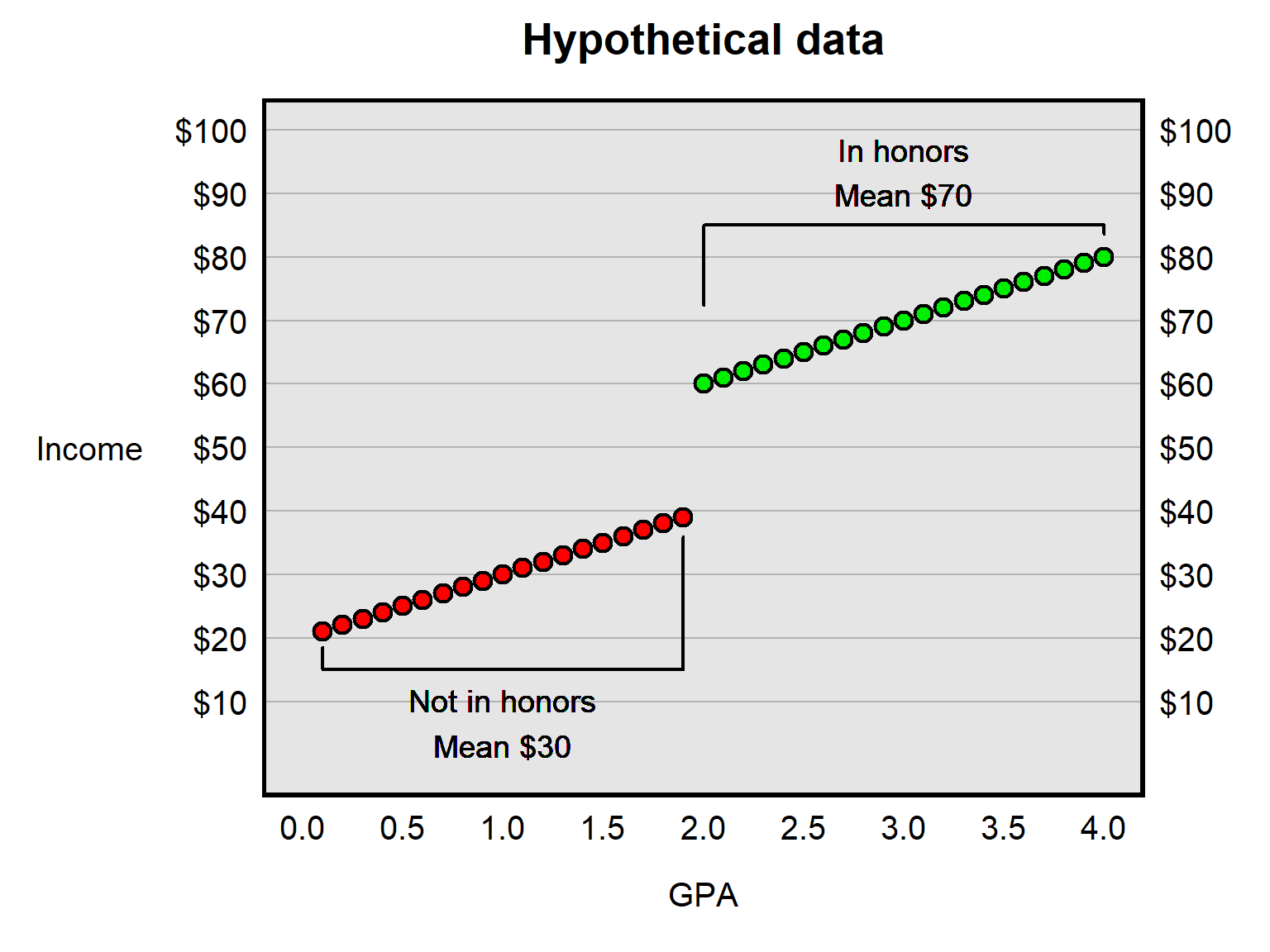
Suppose that we use a discontinuity method to estimate the effect of being in the honors program on future income, by comparing how much income among students who were just below the threshold for getting into the honors program differs from the income among students who were just above the threshold for getting into the honors program. Which of the following best indicates that estimate?
- The honors program reduced income by about $45, on average.
- The honors program reduced income by about $20, on average.
- The honors program did not affect income, on average.
- The honors program increased income by about $20, on average.
- The honors program increased income by about $40, on average.
Answer
- The honors program increased income by about $40, on average.
7.2 Difference-in-differences designs
Suppose that, at Faber College, enrollment in the political science major increased 2% each year from 2012 to 2017. In 2018, the political science department got a new department chair, and, over the next five years, enrollment increased at only 1%. For estimating how the new chair affected enrollment rates in the political science major, which of the following would provide the better comparison for a difference-in-differences design, based on only the enrollment rates indicated below?
- the history major at Faber College, in which enrollment increased at 1% per year from 2012 to 2017
- the sociology major at Faber College, in which enrollment increased at 2% per year from 2012 to 2017
- the economics major at Faber College, in which enrollment increased at 2% per year from 2018 through 2022
Answer
- the sociology major at Faber College, in which enrollment increased at 2% per year from 2012 to 2017
Suppose that a researcher is interested in the extent to which college causes persons to become more politically liberal. In 2019, the researcher surveys a representative sample of age-18 persons who attend college and a representative sample of age-18 persons who do not attend college. Four years later, in 2023, the researcher surveys each person again. Suppose that the researcher’s data are in the table below, in which political ideology is measured from 0 for extremely liberal to 10 for extremely conservative.
                        Mean ideology   Mean ideology
Group                    at age 18       at age 22
------------------------------------------------------
Persons in college          4.5              3.5
Persons not in college      5.0              4.2
If the researcher used a difference-in-differences design that compared persons in college to persons not in college, the researcher’s (more correct) estimate of the effect of college on political ideology would be that college…
- made persons in the sample about 0.2 units more liberal on average
- made persons in the sample about 0.8 units more liberal on average
- made persons in the sample about 1.0 unit more liberal on average
- made persons in the sample about 3.5 units more liberal on average
Answer
- made persons in the sample about 0.2 units more liberal on average
Suppose that, on January 1, 2024, Freedonia enacted the Unemployment Reduction Act. Researchers are interested in assessing the extent to which the Unemployment Reduction Act caused a change in Freedonia’s unemployment rate. Oceania is a country immediately next to Freedonia and is similar to Freedonia in every way, except that Oceania did not enact any legislation to reduce unemployment.
                  Unemployment Rate
             2021   2022   2023   2024
---------------------------------------
Freedonia     6%     6%     6%     3%
Oceania       6%     6%     6%     3%
Considering a difference-in-differences method, what do the data in the table above suggest about the decrease in unemployment in Freedonia between 2023 and 2024?
- The Unemployment Reduction Act was plausibly the reason for the decrease in unemployment in Freedonia between 2023 and 2024.
- The Unemployment Reduction Act was probably not the reason for the decrease in unemployment in Freedonia between 2023 and 2024.
Answer
- The Unemployment Reduction Act was probably not the reason for the decrease in unemployment in Freedonia between 2023 and 2024.
Suppose that unemployment in Freedonia was 12% in 2021, 12% in 2022, and 12% in 2023, and then, on January 1, 2024, Freedonia enacted the Unemployment Reduction Act. Unemployment was then 6% in 2024. Researchers are interested in assessing the extent to which the Unemployment Reduction Act caused this decrease in the unemployment rate. Oceania is a country next to Freedonia and is similar to Freedonia in many ways, but Oceania did not enact any legislation to reduce unemployment.
                  Unemployment Rate
             2021   2022   2023   2024
---------------------------------------
Freedonia     6%     6%     6%     1%
Oceania       6%     6%     6%     6%
Considering a difference-in-differences method, what do the data in the table above suggest about the decrease in unemployment in Freedonia between 2023 and 2024?
- The Unemployment Reduction Act was plausibly the reason for the decrease in unemployment in Freedonia between 2023 and 2024.
- The Unemployment Reduction Act was probably not the reason for the decrease in unemployment in Freedonia between 2023 and 2024.
Answer
- The Unemployment Reduction Act was plausibly the reason for the decrease in unemployment in Freedonia between 2023 and 2024.
7.3 Benchmarks
Membership in the Pi Sigma Alpha national political science honors society requires, among other things, at least a 3.0 GPA. Suppose that we are interested in estimating the effect, if any, that membership in Pi Sigma Alpha has had on the future income of college graduates. Researcher A plans to compare future income among any college students who were in Pi Sigma Alpha to future income among any college students who were not in Pi Sigma Alpha. Researcher B instead plans to compare future income among any college students who were in Pi Sigma Alpha and had a 3.0 GPA to future income among any college students who were not in Pi Sigma Alpha and had a 3.0 GPA. Which researcher has the better research design for estimating the effect, if any, that membership in Pi Sigma Alpha has on the future income of college graduates?
- Researcher A, because Researcher A will have a much larger sample size and thus a more precise estimate of the effect, if any, that membership in Pi Sigma Alpha has on future income.
- Researcher B, because Researcher B’s comparison will better isolate the effect of membership in Pi Sigma Alpha, because both of Researcher B’s groups will be students of similar academic ability.
Answer
- Researcher B, because Researcher B’s comparison will better isolate the effect of membership in Pi Sigma Alpha, because both of Researcher B’s groups will be students of similar academic ability.
Researchers are interested in assessing whether the percentage of women among U.S. political science professors is unfairly too high or too low due to gender bias among the people who hire political science professors. Researcher A plans to compare the percentage of women among U.S. political science professors to the percentage of women among all U.S. residents. Researcher B instead plans to compare the percentage of women among U.S. political science professors to the percentage of women among U.S. residents who have a Ph.D. in political science. Explain why Researcher B’s suggested benchmark might be better than Researcher A’s suggested benchmark.
Answer
People who hire political science professors cannot hire just anyone from the general population but instead must choose from the pool of people who have an advanced degree in political science. The benchmark of the percentage of women among U.S. residents who have a Ph.D. in political science thus better reflects this pool of potential hires.7.4 Panel designs
Suppose that, for two participants, a researcher has data from two surveys, one in April and another in June of the same year. For each participant and for both months, the dataset has an indication of the participant’s political party (D or R) and an indication of whether the participant supports or opposes affirmative action. Data are below, with each participant identified with an ID:
ID       April          June
----------------------------------
1     D + Oppose      D + Support
2     R + Support     R + Oppose
Based on these data only, which of the following is more supported?
- political party influences attitudes about affirmative action
- attitudes about affirmative action influences political party
Answer
- political party influences attitudes about affirmative action
Suppose that, for two participants, a researcher has data from a survey in January and another survey in December of the same year, with each participant appearing twice in the dataset. For each participant and for both months, the dataset has an indication of the participant’s political party (D or R) and an indication of whether the participant supports or opposes affirmative action. Data are below, with each participant identified with an ID:
ID       April          June
----------------------------------
1     D + Oppose      R + Oppose
2     R + Support     D + Support
Based on these data only, which of the following is more supported?
- political party influences attitudes about affirmative action
- attitudes about affirmative action influences political party
Answer
- attitudes about affirmative action influences political party
8.1 Statistical control
How do control variables help improve causal inference in a correlational study?
- reduce bias in measurements
- remove sample bias
- help address alternate explanations
- randomly assign participants
Answer
- help address alternate explanations
In a non-experimental analysis, omission of a relevant control variable…
- can bias an estimate of an effect only to be lower than it truly is
- can bias an estimate of an effect only to be higher than it truly is
- can bias an estimate of an effect to be lower than or higher than it truly is
- cannot bias an estimate
Answer
- can bias an estimate of an effect to be lower than or higher than it truly is
In a non-experimental analysis, including a control variable that should not be included…
- can bias an estimate of an effect only to be lower than it truly is
- can bias an estimate of an effect only to be higher than it truly is
- can bias an estimate of an effect to be lower than or higher than it truly is
- cannot bias an estimate
Answer
- can bias an estimate of an effect to be lower than or higher than it truly is
Suppose that you were asked to conduct a study to determine whether male ISU employees are paid more than female ISU employees are paid. For each ISU employee, you have data on the employee’s salary and their gender. Using these salary data as the outcome, would you need control variables for this study?
- Yes
- No
Answer
- No
Suppose that you were asked to conduct a study to determine whether male ISU employees are unfairly paid more than female ISU employees are paid. For each ISU employee, you have data on the employee’s salary and their gender. Using these salary data as the outcome, would you need control variables for this study?
- Yes
- No
Answer
- Yes
Suppose that, at a certain university, all students must complete an internship. Some students choose to do the internship during the summer, and some students choose to do the internship during the fall or spring. Suppose that we wanted to assess whether completing the internship during the summer causes a student to be more likely or less likely to get a job within a year of graduation, compared to completing the internship during the fall or spring. One problem for our analysis is that the type of student who completes an internship during the summer might differ from the type of student who completes an internship during the fall or spring, and that difference might affect the likelihood that the student gets a job within a year of graduation. Indicate a control variable that can help address this concern, and explain why that control variable can help address this concern.
Answer
Lots of potential acceptable responses, such as the GPA of the student, which might be correlated with selection of the internship time (summer or during the fall or spring) and plausibly influences the likelihood that the student gets a job within six months of graduation.Suppose that you are assigned to test the hypothesis that a female candidate having long hair (compared to having short hair) will affect the percentage of votes that the female candidate receives. For a large set of female candidates, you have data on the percentage of votes that the female candidate received in their election and data on whether that female candidate had long hair or short hair in that election. [1] Identify a control variable that you could use for the analysis. [2] Then explain how that particular control variable would help improve the analysis.
Answer
There are many acceptable responses for this item. One control variable would be the political experience of the female candidate. It is plausible that, in general, a candidate with more political experience should be more likely to win an election (such as a state senator being more likely to be elected to the U.S. senate, compare to a candidate that has no political experience). Therefore, if female candidates who had shorter hair tended to have different levels of political experience than female candidates with longer hair, then any association that we see between hair length and winning an election might be due to the political experience and not the hair length; if we control for hair length, then we have removed hair length as a potential explanation.Below are data on the salary and experience of four male teachers and three female teachers.
Gender   Salary   Experience   Gender   Salary   Experience
 Male      50        Low       Female     50        Low
                               Female     50        Low
 Male      90        High      Female     90        High
 Male      90        High
 Male      90        High
The mean salary among the four male teachers is 80, and the mean salary among the three female teachers is 63.3. Controlling only for experience, the mean salary is…
- the same for male teachers as it is for female teachers
- lower for male teachers than for female teachers
- higher for male teachers than for female teachers
Answer
- the same for male teachers as it is for female teachers
Below are data on the salary and experience of five male teachers and five female teachers.
Gender   Salary   Experience   Gender   Salary   Experience
 Male      60        Low       Female     50        Low
 Male      60        Low
 Male      60        Low
 Male      90        High      Female     80        High
 Male      90        High      Female     80        High
                               Female     80        High
                               Female     80        High
The mean salary among the four male teachers is 72, and the mean salary among the four female teachers is 74. Controlling only for experience, the mean salary is…
- the same for male teachers as it is for female teachers
- lower for male teachers than for female teachers
- higher for male teachers than for female teachers
Answer
- higher for male teachers than for female teachers
8.2 Multiple linear regression
Suppose that researchers are interested in testing whether respondent marital status influences their ratings about the #MeToo movement. The first linear regression below uses data from the ANES 2020 Time Series Study to predict respondent ratings about the #MeToo movement (FTMETOO), using a predictor for respondent marital status. The second linear regression adds a predictor for respondent age.
. reg FTMETOO i.MARITAL
------------------------------------------------------------
       FTMETOO |   Coef.   p-value  [95% Conf. Interval]
---------------+--------------------------------------------
   (intercept) |   55.8    0.000     54.8     56.8
               |
       MARITAL |
      Widowed  |    1.8    0.264     -1.3      4.9
     Divorced  |    4.7    0.000      2.5      6.9
    Separated  |    5.2    0.075     -0.5     11.0
Never married  |    9.9    0.000      8.1     11.8
------------------------------------------------------------

. reg FTMETOO i.MARITAL AGE
------------------------------------------------------------
       FTMETOO |   Coef.   p-value  [95% Conf. Interval]
---------------+--------------------------------------------
   (intercept) |   64.2     0.000      61.2    67.2
               |
       MARITAL |
      Widowed  |    4.1     0.015      0.8      7.5
     Divorced  |    5.1     0.000      2.9      7.3
    Separated  |    5.0     0.096     -0.9     10.8
Never married  |    7.3     0.000      5.2      9.3
               |
           AGE |  -0.1      0.000     -0.2     -0.1
------------------------------------------------------------
Which of the following better indicates the correct interpretation of the 4.1 coefficient for the “Widowed” category in the second regression?
- The predicted difference in FTMETOO between a widowed respondent and a married respondent.
- The predicted difference in FTMETOO between a widowed respondent and a married respondent, controlling for respondent age.
Answer
- The predicted difference in FTMETOO between a widowed respondent and a married respondent, controlling for respondent age.
Suppose that researchers are interested in testing whether respondent marital status influences their ratings about the #MeToo movement. The first linear regression below uses data from the ANES 2020 Time Series Study to predict respondent ratings about the #MeToo movement (FTMETOO), using a predictor for respondent marital status. The second linear regression adds a predictor for respondent age.
. reg FTMETOO i.MARITAL
------------------------------------------------------------
       FTMETOO |   Coef.   p-value  [95% Conf. Interval]
---------------+--------------------------------------------
   (intercept) |   55.8    0.000     54.8     56.8
               |
       MARITAL |
      Widowed  |    1.8    0.264     -1.3      4.9
     Divorced  |    4.7    0.000      2.5      6.9
    Separated  |    5.2    0.075     -0.5     11.0
Never married  |    9.9    0.000      8.1     11.8
------------------------------------------------------------

. reg FTMETOO i.MARITAL AGE
------------------------------------------------------------
       FTMETOO |   Coef.   p-value  [95% Conf. Interval]
---------------+--------------------------------------------
   (intercept) |   64.2     0.000      61.2    67.2
               |
       MARITAL |
      Widowed  |    4.1     0.015      0.8      7.5
     Divorced  |    5.1     0.000      2.9      7.3
    Separated  |    5.0     0.096     -0.9     10.8
Never married  |    7.3     0.000      5.2      9.3
               |
           AGE |  -0.1      0.000     -0.2     -0.1
------------------------------------------------------------
Explain a benefit of the second regression controlling for respondent age.
Answer
Respondents who have different marital statuses might have different ages on average; for example, in the ANES 2020 Time Series Study, the average age for married respondents was 54, but the average age for widowed respondents was 71. If we want to better isolate the effect of marital status, we can compare respondents with different marital statuses at the same age. So, for example, instead of comparing the average married respondent (age 54) to the average widowed respondent (age 71), we would compare a married respondent at age 54 to a widowed respondent at age 54, and then compare a married respondent at age 55 to a widowed respondent at age 55, and so forth, and then average these comparisons.8.3 Illustration of the effects of statistical control
Answer
The plot below reports on the x-axis whether the police officer wears a body camera (0 for No, and 1 for Yes) and on the y-axis the number of complaints received by a police officer. The color of the points indicates the officer’s age, with black being age 20, gray being age 30, and white being age 40. The slope of the line in the plot is the association between X and Y without any controls, suggesting that the body camera associates with 5.2 fewer complaints on average.
If we predict complaints using the bodycam variable and a control for the age of the officer, that analysis will suggest that the body camera associates with ___. A. 5.2 fewer complaints on average B. less than 5.2 fewer complaints on average C. more than 5.2 fewer complaints on average
For each age (colored black, gray, and white), the line of best fit is flat. This flat line suggests that – controlling for age – the body cam did not affect the number of complaints.
9.1 Peer review
In political science, for peer review of papers that report a statistical analysis, is it typical for the peer reviewers to check the data to see whether the statistical analysis has been correctly conducted?
- Yes
- No
Answer
- No
Which of the following is the “blind” element of single-blind peer review of a paper?
- Peer reviewers are not told the names of the paper’s authors
- Authors are not told the names of the peer reviewers
Answer
- Authors are not told the names of the peer reviewers
9.2 Pre-registration
Franco et al. 2014 found that null results were ___ likely to be published than strong results were to be published.
- much less
- just as
- much more
Answer
- much less
Of the following, which term best describes the process in which researchers publicly post ahead of time a plan for the research that they will conduct?
- Premonition
- Replication
- Pre-registration
- Post-registration
Answer
- Pre-registration
9.3 Meta-analysis
Study A has an estimated effect of 10 units and a sample size of 100 participants. Study B has an estimated effect of 2 units and a sample size of 200 participants. Which study should receive more weight in a meta-analysis?
- Study A, because Study A has a larger estimated effect size
- Study B, because Study B has a larger sample size
Answer
- Study B, because Study B has a larger sample size
Below are data for two studies:
       Estimated
        effect     Sample
Study    size      size
--------------------------
  A       2         300
  B       5         200
Which of the following is a correct formula for calculating the mean estimated effect size, weighted by sample size?
- 2 \(\times\) (300) + 5 \(\times\) (200)
- 2 \(\times\) (300 \(\div\) 200) + 5 \(\times\) (200 \(\div\) 300)
- 2 \(\times\) (300 \(\div\) 500) + 5 \(\times\) (200 \(\div\) 500)
- 300 \(\times\) (2 \(\div\) 7) + 200 \(\times\) (5 \(\div\) 7)
Answer
Explain why a meta-analysis might be better than a single well-done study as a source for information about a research question.
Answer
Meta-analyses collect data from multiple studies, so these meta-analyses should have larger sample sizes than an individual study in the meta-analysis and thus have more information. Moreover, meta-analyses collect data from different studies, so any particular idiosyncrasy from a study should hopefully even out or be overpowered when combined with other studies.A meta-analysis can use all studies available on a research question to produce an average estimate from these studies. Explain the benefit of the meta-analysis average being weighted by sample size.
Answer
Compared to studies that have a smaller sample, studies that have a larger sample have more data and typically provide more information about the research question, so these larger sample studies should receive more emphasis in the meta-analysis than the smaller sample studies receive.Explain why a meta-analysis might be better than a single well-done study as a source for information about a research question.
Answer
Meta-analyses collect data from multiple studies, so these meta-analyses should have larger sample sizes than an individual study in the meta-analysis and thus have more information. Moreover, meta-analyses collect data from different studies, so any particular idiosyncrasy from a study should hopefully even out or be overpowered when combined with other studies.10.1 Selection bias
Suppose that, for a POL 138 course, the instructor gives a pretest at the first class meeting and then gives the same test as a posttest at the last class meeting before the final exam. Each of the 100 students registered for the course attended the first class meeting and took the pretest, but the instructor did not require attendance, and only 60 of the 100 students attended the final class meeting before the final exam and took the posttest. For the 60 students who took both the pretest and the posttest, results indicated that, on average, these students increased their pretest score by 20% from the pretest to the posttest. But, for the final exam taken by all 100 students, the increase in score was only 12% on average. Of the following, which is the most plausible reason that the pretest/posttest comparison overestimated the amount of learning in the class, compared to the estimated learning from the final exam?
- Kelley’s paradox
- Regression toward the mean
- Selection bias
- Simpson’s paradox
Answer
- Selection bias
The SAT test is optional in Pennsylvania, and only 48% of Pennsylvania high school students in the class of 2023 took the SAT. The mean SAT score among these students was 1078. Suppose that Pennsylvania had instead required that all high school students in the class of 2023 take the SAT. Indicate whether you expect the mean SAT score among all Pennsylvania students in the class of 2023 to have been 1078, lower than 1078, or higher than 1078, if all Pennsylvania students took the SAT. Then explain why.
Answer
One possible response that would get credit: It seems plausible that students who took the SAT are, on average, better students who would be expected to score higher on the SAT, compared to students who did not take the SAT. If so, then the expectation is that the mean SAT score among all Pennsylvania students in the class of 2023 is lower than 1078.10.2 Per capita
Suppose that the island country of Madripoor has 200,000 native residents and 50,000 immigrants. In 2023, 300 native Madripoor residents and 100 immigrants to Madripoor were a victim of a hate crime.
There were more hate crimes against…
- immigrants to Madripoor
- native Madripoor residents
Answer
- native Madripoor residents
Suppose that the island country of Madripoor has 200,000 native residents and 50,000 immigrants. In 2023, 300 native Madripoor residents and 100 immigrants to Madripoor were a victim of a hate crime.
The per capita rate of being a victim of a violent crime was higher among…
- immigrants to Madripoor
- native Madripoor residents
Answer
- immigrants to Madripoor
per capita calculations:
300 \(\div\) 200,000 compared to 100 \(\div\) 50,000, which is equivalent to 0.0015 compared to 0.0020Suppose that, at the start of 2020, Freedonia had 1,000 Asian residents and 3,000 Black residents. During 2020, covid caused the death of 100 of these Asian residents and 200 of these Black residents. Which group had a higher per capita rate of death from covid-19 in 2020?
- Asian residents of Freedonia
- Black residents of Freedonia
Answer
- Asian residents of Freedonia
Per capita calculations:
- Asian = 100 \(\div\) 1,000 = 0.10
- Black = 200 \(\div\) 3,000 = 0.07
10.4 Using a less relevant measure
The Bone Student Scholar award is the most prestigious undergraduate student award at Illinois State University and is given to students who have at least four semesters at ISU and who have a cumulative GPA of at least 3.7. For the 2021-2022 school year, 14 students were named a Bone Student Scholar. Nine of these 14 students were female (64%). To assess the extent to which this percentage is fair, which of the following pieces of information would be more useful to know?
- the percentage of female students among all ISU students
- the percentage of female students among all ISU students who have at least four semesters at ISU and who have a cumulative GPA of at least 3.7
Answer
- the percentage of female students among all ISU students who have at least four semesters at ISU and who have a cumulative GPA of at least 3.7
Suppose that each public high school in Illinois selects their three best math students to represent the school in a competition answering math questions. For each student, we have data on the student’s score on the most recent state standardized math test. EXPLAIN which one of the following would be most useful for predicting which school will win the competition:
- the 1st percentile score for each school on the state standardized math tests
- the mean score for each school on the state standardized math tests
- the median score for each school on the state standardized math tests
- the 99th percentile score for each school on the state standardized math tests
Answer
The 99th percentile score is the score under which 99 percent of scores fall; students at the 99th percentile are the highest scoring students, among the options available in the item. So, the higher this 99th percentile score is for a school, the better the best students at the school have performed on the standardized math tests. For this item, we are interested in the performance of the best students at each school, so, of the options, that 99th percentile score for each school would provide the best sense of how the best students in one school compare to the best students in the other schools.Suppose that the political science department at Faber College administers a political science knowledge test to all of its political science majors. The department issues a “political science expert” award only to the ten students who have the ten highest scores on the political science knowledge test. For this test, the mean score among the 500 female political science majors was 50, and the mean score among the 500 male political science majors was 40, but the department gave 7 of the 10 “political science expert” awards to male political science majors. Explain how male political science majors could fairly receive the majority of the “political science expert” awards if female political science majors had a higher mean score on the test than male political science majors did.
Answer
The “political science expert” awards were given to students at the high end of the distribution of the test, so it is possible that the scores among male political science majors had a higher standard deviation than the scores among female political science majors.10.5 Measurement error
Suppose that, over the past ten years, the reported number of burglaries has substantially decreased in Freedonia City. One possible explanation for this is that prevalence of burglary has decreased. But what else might this be due to?
Answer
Another potential explanation is that merely the reporting of the burglaries has decreased. Maybe, for instance, it has become well known that police have not recently investigated or solved many burglaries, so that a lot of people don’t bother to report burglaries. In that case, the reported number of burglaries could decrease even if the number of burglaries has not decreased.10.6 Restriction of range
Suppose that researchers test whether political science majors know more about politics on average than business majors know. Researchers claim that, in their data, political science majors do not know more about politics on average than business majors know. One explanation for this finding is that, in reality, political science majors do not know more about politics on average than business majors know. But explain how this finding might merely have been due to restriction of range in the researchers’ research design.
Answer
The test that researchers used to measure knowledge about politics might have been so easy or so difficult that the test was not able to detect a true difference of knowledge about politics, on average, between political science majors and business majors.10.7 Confounders
Suppose that an analysis indicated that, in head-to-head matchups between major party candidates in the United States, the candidate that raises more money wins in 90% of elections. Suppose also that the p-value is p<0.05 for a test of the null hypothesis that the candidate that raised more money was just as likely to win election as the candidate that raised less money. Explain whether this would be sufficient evidence at the conventional level of political science to conclude that raising more money than the other candidate causes a candidate to be more likely to win an election.
Answer
No, because there are reasonable alternate explanations that must first be addressed. For example, maybe candidates who are winning in the polls are more likely to receive campaign donations because they are winning in the polls. In that case, the chance of winning causes the donations and not vice versa.10.8 Miscontrolling
Suppose we test whether variation in X causes variation in Y. Which of the following would be worse to add as a predictor to that regression?
- a variable A that influences X and influences Y
- a variable B that is influenced by X and is influenced by Y
Answer
- a variable B that is influenced by X and is influenced by Y
Omission of a relevant control variable in a non-experimental analysis…
- cannot bias an estimate of an effect
- can bias an estimate of an effect only to be lower than it truly is
- can bias an estimate of an effect only to be higher than it truly is
- can bias an estimate of an effect to be lower than or higher than it truly is
Answer
- can bias an estimate of an effect to be lower than or higher than it truly is
Inclusion of an irrelevant control variable in a non-experimental analysis can…
- cannot bias an estimate of an effect
- can bias an estimate of an effect only to be lower than it truly is
- can bias an estimate of an effect only to be higher than it truly is
- can bias an estimate of an effect to be lower than or higher than it truly is
Answer
- can bias an estimate of an effect to be lower than or higher than it truly is
11.1 Misinterpreting p>0.05
Sometimes a research study does not permit an inference that the effect of a treatment differs from zero; these inconclusive studies can be referred to as producing a null result. An “informative null” can be used to refer to a study that had a null result but nonetheless provided information that the treatment effect is at most small. Of the measures below, which measure is most useful for assessing whether a result from a study can be appropriately referred to as an informative null?
- a p-value
- a standard deviation
- a 95% confidence interval
Answer
- a 95% confidence interval
Suppose that researchers in Latveria are interested in whether married men have a different income on average than never married men have. For a representative sample of Latverian men, the researchers compare the mean income of married Latverian men to the mean income of never married Latverian men. The p-value is p=0.25 for a test of the null hypothesis that these means equal each other. Which of the 95% confidence intervals below for the difference in mean incomes would be a more informative null?
- [-$200, +$300]
- [-$40,000, +$40,000]
Answer
- [-$200, +$300]
Misinterpreting differences in statistical significance
Amy flips her coin a certain number of times, and Bob flips his coin a different number of times. Amy and Bob then each test the null hypothesis that their coin is fair. Amy’s p-value is p=0.04, and Bob’s p-value is p=0.50. Is this sufficient evidence to conclude at the conventional level in political science that Amy’s coin is less fair than Bob’s coin?
- Yes
- No
Answer
- No
Suppose that researchers test the effect of a treatment. Results provide evidence at p=0.03 that the treatment worked among men participants, but the p-value is p=0.20 for the test of the effect among women participants. Is this sufficient evidence to support the conclusion that the treatment was more effective among men participants than among women participants?
- Yes: the p-values of p=0.03 and p=0.20 provide sufficient evidence that the treatment worked among men participants but did not provide sufficient evidence that the treatment worked among women participants.
- No: p-values do not directly indicate anything about effect sizes, so we cannot conclude based on these p-values that the effect size was larger for men participants than for women participants.
Answer
- No: p-values do not directly indicate anything about effect sizes, so we cannot conclude based on these p-values that the effect size was larger for men participants than for women participants.
11.3 Multiple testing
Suppose that Researcher A and Researcher B independently test whether a treatment has an effect. Researcher A conducts a randomized experiment with a sample size of 800, to assess whether the treatment has an effect. Researcher B conducts a different randomized experiment with a sample size of 1600, to assess whether the treatment has an effect. Researcher A and Researcher B then each use their data to test the null hypothesis that the treatment has no effect. In reality, the treatment has no effect. What is the expected probability that at least one of these experiments produced a p-value of 0.05 or less?
- 0%
- above 0% but less than 5%
- 5%
- above 5% but less than 50%
- 50%
- above 50% but less than 95%
- 95%
- above 95% but less than 100%
- 100%
Answer
- above 5% but less than 50%
11.4 Regression toward the mean
Suppose that data from the Freedonia Department of Transportation indicate that the number of traffic crash fatalities from 2016 through 2022 had been 978, 990, 935, 910, 996, and 1134. After the jump from 996 fatalities to 1134 fatalities, Freedonia state troopers began a program to more frequently ticket speeding vehicles. The next year, the number of traffic crash fatalities fell from 1134 to 960. Using these data to conclude that the new ticketing policy caused the drop from 1134 to 960 best reflects a lack of consideration of which of the following?
- an ecological fallacy
- Kelley’s paradox
- regression toward the mean
- Simpson’s paradox
Answer
- regression toward the mean
11.6 Simpson’s paradox
Suppose that, in group A, men are on average older than women are. Suppose that, in group B, men are on average older than women are. If group A and group B are combined into group C, then, in group C, …
- men will be older on average than women are
- men will not necessarily be older on average than women are
Answer
- men will not necessarily be older on average than women are
11.7 Heterogenous effects
Suppose that we conduct a randomized experiment to estimate the effect of a treatment, but we do not detect sufficient evidence that the treatment differs from zero. One potential reason for this null result is heterogeneous effects, which refers to…
- socially desirable effects
- effects that differ between subpopulations
- effects that regress toward the mean
Answer
- effects that differ between subpopulations
11.9 Lack of external validity
Validity refers to the extent to which a measuring tool…
- produces consistent results
- produces statistically significant results
- measures what the tool is supposed to measure
Answer
- measures what the tool is supposed to measure
Which type of validity concerns the ability of a research result to generalize to the population?
- internal validity
- external validity
Answer
- external validity
Which type of validity concerns the ability to make correct claims about the sample?
- internal validity
- external validity
Answer
- internal validity
Suppose that a researcher tests for racial bias. The researcher conducts a randomized experiment in which a large sample of students from the local college are randomly given a story about a Black man convicted of a DUI or a White man convicted of a DUI. Everything else in the story is the same, except for the race of the man convicted of a DUI. The researcher analyzes the responses to see whether the mean sentence length recommended for the Black man convicted of a DUI differs from the mean sentence length recommended for the White man convicted of a DUI. Does this study have a high amount of internal validity?
- Yes, because the study is a randomized experiment that manipulated only the man’s race.
- Yes, because the study has a large sample.
- No, because college students are plausibly not representative of persons in the legal system who will decide in real life the sentence length for a DUI.
- No, because the study did not have enough control variables to eliminate all plausible alternate explanations.
Answer
- Yes, because the study is a randomized experiment that manipulated only the man’s race.
Suppose that a researcher tests for racial bias. The researcher conducts a randomized experiment in which a large sample of students from the local college are randomly given a story about a Black man convicted of a DUI or a White man convicted of a DUI. Everything else in the story is the same, except for the race of the man convicted of a DUI. The researcher analyzes the responses to see whether the mean sentence length recommended for the Black man convicted of a DUI differs from the mean sentence length recommended for the White man convicted of a DUI. Does this study have a high amount of external validity?
- Yes, because the study is a randomized experiment that manipulated only the man’s race.
- Yes, because the study has a large sample.
- No, because college students are plausibly not representative of persons in the legal system who will decide in real life the sentence length for a DUI.
- No, because the study did not have enough control variables to eliminate all plausible alternate explanations.
Answer
- No, because college students are plausibly not representative of persons in the legal system who will decide in real life the sentence length for a DUI.
11.10 Researcher bias or researcher error
Suppose that results from a large sample random representative survey of U.S. residents indicates that the percentage of Republicans who agree with the statement that “Covid-19 is less dangerous than the flu” is higher than the percentage of Democrats who agree with that statement, with a p-value of p<0.05 for a test of the null hypothesis that these percentages equal each other. Presuming that it is not true that covid-19 is less dangerous than the flu, are these data sufficient to conclude that, at least at the time of the survey, the percentage of Republicans in the United States who were misinformed about the severity of covid-19 is higher than the percentage of Democrats in the United States who were misinformed about the severity of covid-19?
- Yes
- No
Answer
- No
12.1 IRBs
IRBs are organizations designed to protect human subjects in scientific research. Can an IRB, in some circumstances, permit research involving human participants in which the human participants do not provide informed consent?
- Yes
- No
Answer
- Yes
12.2 Statistical discrimination
Discrimination in which unknown information for an individual is estimated based on known or perceived data for the individual’s group is referred to as…
- statistical discrimination
- taste-based discrimination
Answer
- statistical discrimination
12.3 Kelley’s paradox
Suppose that, for a multiple-choice political science knowledge test, students from State A have a mean score of 40 and students from State B have a mean score of 60. Scores in both states follow a normal distribution, and the standard deviation of scores in both states is 10. Because of Kelley’s paradox, a randomly selected student from State A who has a score of 80 will be expected to be more likely to have ___ true level of political science knowledge than a randomly selected student from State B who has a score of 80.
- a lower
- the same
- a higher
Answer
- a lower
Practice open-ended items
Suppose that we are assessing whether there is a “pink tax”, in which the version of a product marketed to women unfairly costs more than the equivalent version of the product marked to men. Our analysis involves only two products: a $10 pack of 10 men’s razor blades, and a $6 pack of 5 women’s razor blades. The men’s razor blades cost an average of $1.00 each, but the women’s razor blades cost an average $1.20 each. Indicate one thing that we should consider before concluding that, in comparing these two products, this 20-cent difference in average price per razor blade is sufficient evidence that the razor blades marketed to women unfairly cost more on average than the razor blades marketed to men cost. Then explain why.
Answer
One potential response that would receive full credit: Before concluding that the 20 cent difference in average price per razor blade is sufficient evidence that the razor blades marketed to women unfairly cost more on average than the razor blades marketed to men cost, we should consider the fact that the women’s razor blades might be higher quality than the women’s razor blades (such as stronger materials or a sharper blade) and thus the 20 cent difference is fair.
Another idea is that, because men typically shave more often than women, it’s reasonable for the men’s package to have more razor blades, and it’s also reasonable to discount purchases in bulk (i.e., giving a discount for buying more razor blades per pack), so that it’s fair that men pay less than women for each razor blade.Explain what information a p-value provides. Then indicate which p-value represents no evidence against the null hypothesis, which p-value represents infinitely strong evidence against the null hypothesis, and what the conventional p-value threshold is in political science.
Answer
A p-value is a measure of the strength of evidence that an analysis has provided against the null hypothesis. A p-value of 1 represents no evidence against the null hypothesis, a p-value of 0 represents infinitely strong evidence against the null hypothesis, and p=0.05 is the conventional p-value threshold in political science.Suppose that an analysis indicated that, in head-to-head matchups between major party candidates in the United States, the candidate who raises more money wins in 90% of elections. Suppose also that the p-value is p<0.05 for a test of the null hypothesis that the candidate that raised more money was just as likely to win election as the candidate that raised less money. Explain whether this would be sufficient evidence at the conventional level of political science to conclude that raising more money than the other candidate causes a candidate to be more likely to win an election.
Answer
Not sufficient evidence, because there are alternate explanations that should be addressed. For example, maybe the candidate that raises more money was more likely to be an incumbent, and this incumbency caused the candidate to be more likely to win an election.Suppose that an analysis indicated that, in the United States, political candidates who wear an American flag pin are more likely to win their election, compared to political candidates who do not wear an American flag pin. Suppose that the p-value is p<0.05 for a test of the null hypothesis that political candidates who wear an American flag pin are just as likely to win their election as political candidates who do not wear an American flag pin. Identify one control variable that this analysis should include before we conclude that, at least on average in the United States, wearing an American flag pin causes a political candidate to be more likely to win their election. Then explain why that control variable would be useful for this analysis.
Answer
One control variable would be whether the candidate is an incumbent. It’s possible that – compared to candidates who don’t wear an American flag pin – candidates who wear an American flag pin are more (or less) likely to be an incumbent, and a control variable for incumbency can help isolate the effect of the flag pin from the effect of incumbency.Suppose that we conducted a randomized experiment in which a random sample of U.S. residents watched a video of a political candidate’s speech. Some participants were randomly assigned to a video in which the candidate wore an American flag pin, and other participants were randomly assigned to a video in which the same candidate did not wear an American flag pin. Everything else was the same between these videos, except for the American flag pin. After the video, all participants indicated on a scale from 0% to 100% the probability that the participant would vote for the candidate. Results indicated that the mean probability was 10 percentage points higher among participants who were randomly assigned to watch the video in which the candidate wore an American flag pin, compared to the mean probability among participants who were randomly assigned watch to the video in which the candidate did not wear an American flag pin, with a p-value of p<0.05 for a test of the null hypothesis that these mean probabilities equaled each other. Explain why this randomized experiment might be better for assessing whether wearing an American flag pin causes a political candidate to be more likely to win their election, compared to the non-experimental research study described in the prior item.
Answer
Everything else was the same between the videos, except for the American flag pin, so the only reasons for a difference between groups would be the American flag pin or random assignment error. The p-value for a test of the null hypothesis was p<0.05, so we can eliminate random assignment error as a plausible explanation. Thus, the only plausible explanation remaining is the American flag pin. This randomized experiment is better than the non-experimental research study described in Question 3, because the “flag pin” candidates in the non-experimental research study might not have been all else equal to the “no flag pin” candidates, and these other differences might have caused the observed difference in winning the election.Suppose that, for the randomized experiment in the prior item, the p-value was p=0.24 for the test of the null hypothesis. Explain one way that that null result could occur, if it were true that wearing an American flag pin causes a political candidate to be more likely to win their election. Possible reasons include random assignment error, restriction of range, a too small sample size, and inattentive participants. Don’t merely select one of these reasons: Select a reason, and then explain how that could cause the null result.
Answer
One potential response that would receive full credit: The null result could have been caused by a too small sample size. Small sample sizes don’t provide much information about the effect that we are testing for, so it’s possible that a randomized experiment with a small sample size merely did not detect an effect that exists.Suppose that, at a certain university, students must complete an internship during the summer of their junior year or during the fall of their senior year. Some students choose to complete the internship during the summer of their junior year, and some students choose to complete the internship during the fall of their senior year. Suppose that students who complete the internship during the fall of their senior year are more likely to get a job within a year of graduation, compared to students who complete the internship during the summer of their junior year. One potential reason for this difference is that employers prefer to hire students who have completed their internship more recently so that the letters of recommendation are more recent. Provide one other possible reason that might explain why students who complete the internship during the fall of their senior year are more likely to get a job within a year of graduation, compared to students who complete the internship during the summer of their junior year.