1 Basic tools of quantitative reasoning
1.1 Quantitative reasoning
Quantitative reasoning focuses on understanding the world through numbers. This course is designed to improve your ability at quantitative reasoning.
Some things that we’d like to improve your ability at are:
- understanding how quantitative analyses can help measure characteristics of a population,
- understanding how quantitative analyses can help determine what causes what,
- understanding how quantitative analyses might be misleading due to error or intentional bias,
- using software to perform quantitative analyses
This course is about quantitative reasoning in political science, but the concepts that we discuss can be applied to other areas of life, to help us assess evidence for questions such as:
- Should I take a particular medicine?
- Does breastfeeding improve child outcomes?
- Do any benefits of breastfeeding a child persist into adulthood?
- How large are any breastfeeding benefits that persist into adulthood?
This course will focus on making correct inferences. An inference is a conclusion about something that is not observed, based on things that are observed. For example, we might make a conclusion about the 350 million or so U.S. residents, based on a sample of only 3,000 U.S. residents. Causal inference is about what causes what, such as the extent, if any, to which a U.S. resident’s preferences about gun policy influence their vote for U.S. president. Descriptive inference does not concern causality. A sample descriptive inference question might be the percentage of the U.S. population that supports a ban on guns.
Let’s discuss some basic tools of quantitative reasoning…
1.2 Measures of central tendency
Major learning objective(s) for this section:
- Determine the mean of a set of data.
- Determine the median of a set of data.
Measures of central tendency provide information about the center of a set of numbers. A common measure of central tendency is the mean, which is the sum of all of the numbers in the set, divided by the total number of numbers in the set. Another common measure of central tendency is the median, which is a number that divides in half a set of numbers that is ordered from low to high. If the ordered set of numbers has an odd number of numbers, the median is the middle number; if the ordered set has an even number of numbers, the median is the mean of the middle two numbers.
Consider the set of five numbers {0,0,1,9,90}:
- The mean is (0+0+1+9+90) \(\div\) 5, which is 100 \(\div\) 5, which is 20.
- The median is the middle number in the ordered set, which is 1.
For another example, consider the set of six numbers {0,0,0,1,9,90}:
- The mean is (0+0+0+1+9+90) \(\div\) 6, which is about 16.7.
- The median is the mean of the middle two numbers in the ordered set, which is (0+1) \(\div\) 2, or 0.5.
Sample practice items
What is the mean of the set of numbers {0,10,20,70}?
Answer
(0+10+20+70) \(\div\) 4, which is 25What is the median of the set of numbers {0,5,19}?
Answer
5, which is the middle number when the set is ordered from low to highWhat is the median of the set of numbers {0,10,20,70}?
Answer
15, which is the mean of the two middle numbers (10 and 20) when the set is ordered from low to high1.3 Outliers
Major learning objective(s) for this section:
- Know what an outlier is, and estimate the effect of an outlier.
An outlier is a number in a set that is very far away from most of the other numbers in the set. A set of numbers might have no outliers, such as {-1,0,1,2,3,4}. Or a set of numbers might have one outlier, such as {0,0,0,1,9,90}, in which 90 is an outlier. Or a set of numbers might have multiple outliers, such as in the set {-100,-99,0,0,0,0,0,0,0,0,0,0,0,0,1,1,1,1,1,1,1,1,2,2,80}, in which -100, -99, and 80 are outliers.
An outlier affects the mean of a set of numbers more than an outlier affects the median of a set of numbers. For example, for the set {0,1,2}, the mean is 1, and the median is 1. But if we add the outlier 97 to get the set {0,1,2,97}, the mean increases to 25, but the median increases only to 1.5. Sometimes the mean can be a more useful measure than the median, and sometimes the median can be a more useful measure than the mean: it depends on whether outliers should have a small influence (in which case, the median is more useful) or a large influence (in which case, the mean is more useful).
Sample practice items
Which, if any, numbers is or are an outlier in the set {-1, 0, 0, 1, 1001}?
Answer
1001 onlyAdding an outlier to a set of numbers is expected to cause a bigger change to ___ of the set of numbers.
- the mean
- the median
Answer
- the mean
Removing an outlier from a set of numbers is expected to cause a bigger change to ___ of the set of numbers.
- the mean
- the median
Answer
- the mean
A set of data for a research study indicated that international relations articles written by women received a higher median number of citations than international relations articles written by men did. Does this necessarily indicate that this set of data would also indicate that international relations articles written by women received a higher mean number of citations than international relations articles written by men did?
- Yes
- No, not necessarily
Answer
- No, not necessarily
If men were more likely than women to have an outlier high number of citations, then that could push the male mean above the female mean, even if women had a higher median number of citations than men did. Consider the example in which citations are {0,1,98} for men and are {2,2,2} for women. The median is 1 for men and 2 for women, so the median is higher for women. But the mean is 33 for men, which is higher than the mean of 2 for women.
1.4 Standard deviation
Major learning objective(s) for this section:
- Answer items measuring knowledge of the definition of a standard deviation.
For a set of numbers, the standard deviation measures the typical distance between a number in the set and the mean of the set: all else equal, the more closely clustered the points are around the mean, the smaller the standard deviation is. Standard deviations range from 0 (if all numbers in the set are at the mean of the set) to infinity (for infinitely large dispersion around the mean). See the plot below for some examples.
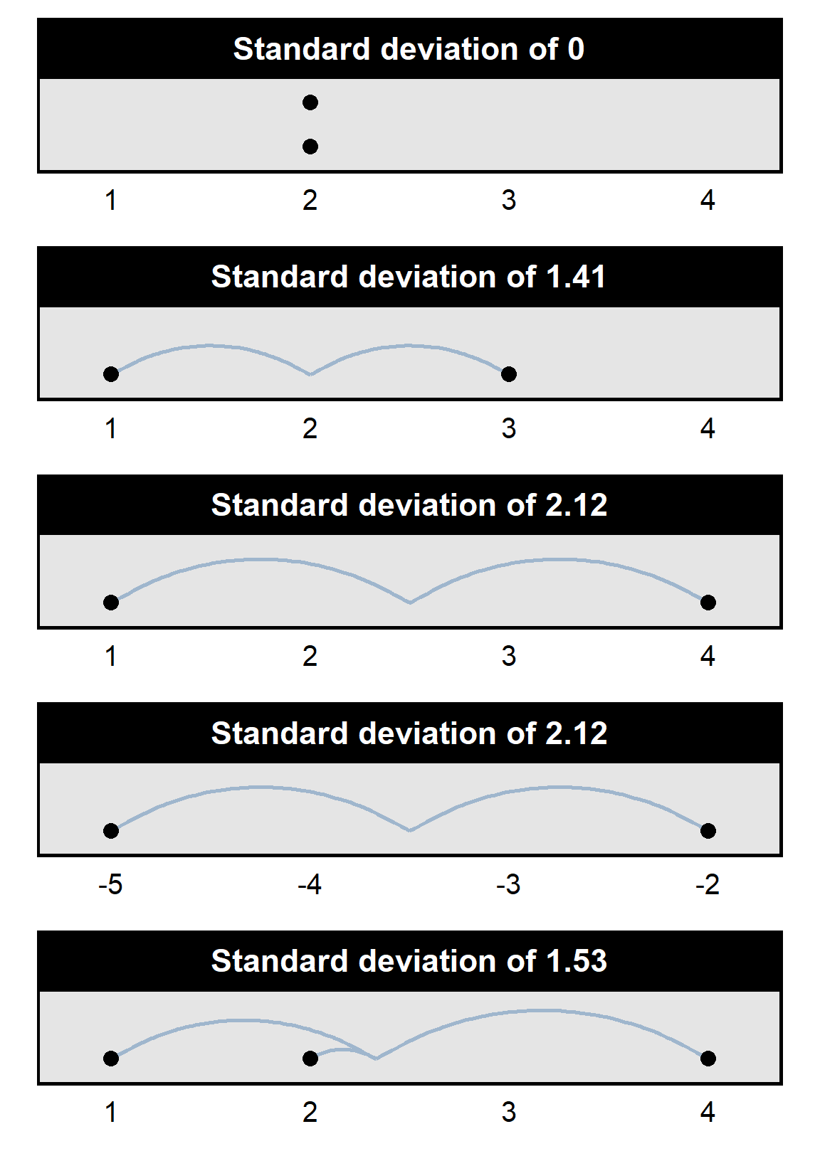
As indicated in the plot above, the standard deviation of the set {2,2} is 0, the standard deviation of the set {1,3} is 1.41, and the standard deviation of the set {1,4} is 2.12. And the standard deviation is also 2.12 for the set of numbers {-5,-2}, even though each number in the set is negative: standard deviation measures variation around the mean, and the numbers in the set {-5,-2} have just as much variation around the mean as the numbers in the set {1,4} have.
Standard deviation is not the same as the range: the standard deviation of the set {1,4} is 2.12, but the standard deviation of the set {1,2,4} is 1.53, because the average variation around the mean for the set of numbers {1,2,4} is less than the average variation around the mean for the set of numbers {1,4}.
Students will not need to calculate a standard deviation in this POL 138 course, but students are expected to correctly respond to items about the fact that standard deviation measures the variation that a set of numbers has around the mean of the set of numbers.
Sample practice items
For a set of numbers, the standard deviation is a measure of…
- central tendency
- correctness
- reliability
- validity
- variation
Answer
- variation
Which of the following correctly describes the standard deviation of the set of numbers {0,10,20}?
- The standard deviation is less than zero.
- The standard deviation is zero.
- The standard deviation is greater than zero.
Answer
- The standard deviation is greater than zero.
Standard deviation measures variation, and there is some variation in the set of numbers.
Which of the following correctly describes the standard deviation of the set of numbers {-2,-4,-6}?
- The standard deviation is less than zero.
- The standard deviation is zero.
- The standard deviation is greater than zero.
Answer
- The standard deviation is greater than zero.
Standard deviation measures variation, and there is some variation in the set of numbers.
Which of the following correctly describes the standard deviation of the set of numbers {-3,-3,-3}?
- The standard deviation is less than zero.
- The standard deviation is zero.
- The standard deviation is greater than zero.
Answer
- The standard deviation is zero.
Standard deviation measures variation, and there is no variation in the set of numbers.
Suppose that the weight of six students weights in pounds are: {150, 160, 180, 185, 200, 220}. The standard deviation of these six numbers is 25.6. Suppose that each participant was wearing 5 pounds of clothes, so we subtract 5 pounds from each measurement to get these weights: {145, 155, 175, 180, 195, 215}. What would be the standard deviation for the new weights?
- Less than 25.6 pounds
- 25.6 pounds
- Greater than 25.6 pounds
Answer
- 25.6 pounds
Subtracting 5 pounds does not change the amount of variation in the set of numbers. Each number shifts 5 lower, but the numbers don’t get closer to each other or farther from each other.
Suppose that a teacher gave an exam with 100 questions. The mean number of questions correct was 60, and the standard deviation for the number of questions correct was 20. Each question correct on the exam was worth 2 points. What is the standard deviation of the set of points earned, or is it not possible to know the standard deviation without additional information?
- Less than 20 points
- 20 points
- Greater than 20 points
- It is not possible to know the new standard deviation without additional information
Answer
- Greater than 20 points
Multiplying numbers by 2 spreads the numbers farther out. Consider the numbers correct of 10 and 11, which are 1 apart. Counting those as 20 points and 22 points makes those 2 units apart, and thus the variation in the set of the numbers is farther apart.
Suppose that the statistics for a 100-point final exam in a particular course were a mean of 60 and a standard deviation of 10, and a range from a low of 0 to a high of 90. Suppose that the teacher added 10 points to each score, so that the new mean is 70 and the new range is from 10 to 100. What is the standard deviation of the new set of scores, or is it not possible to know the new standard deviation without additional information?
- Less than 10 points
- 10 points
- Greater than 10 points
- It is not possible to know the new standard deviation without additional information
Answer
- 10 points
Adding 10 to each score did not spread the scores out any farther than the scores were before.
What would you expect about the standard deviation the set of eight numbers in the bottom row of the table below?
- The standard deviation is 0.534.
- The standard deviation is less than 0.534.
- The standard deviation is greater than 0.534.
Set of            Standard
eight numbers     deviation
---------------------------
0,0,0,0,0,0,0,0   0.000
0,0,0,0,0,0,0,1   0.353
0,0,0,0,0,0,1,1   0.463
0,0,0,0,0,1,1,1   0.517
0,0,0,0,1,1,1,1   0.534
0,0,0,1,1,1,1,1   ?
Answer
The standard deviation for the missing row will be the same as the standard deviation for {0,0,0,0,0,1,1,1}, which is 0.517. The {0,0,0,0,0,1,1,1} and {0,0,0,1,1,1,1,1} have numbers just as far from each other.1.5 Histograms
Major learning objective(s) for this section:
- Read a histogram.
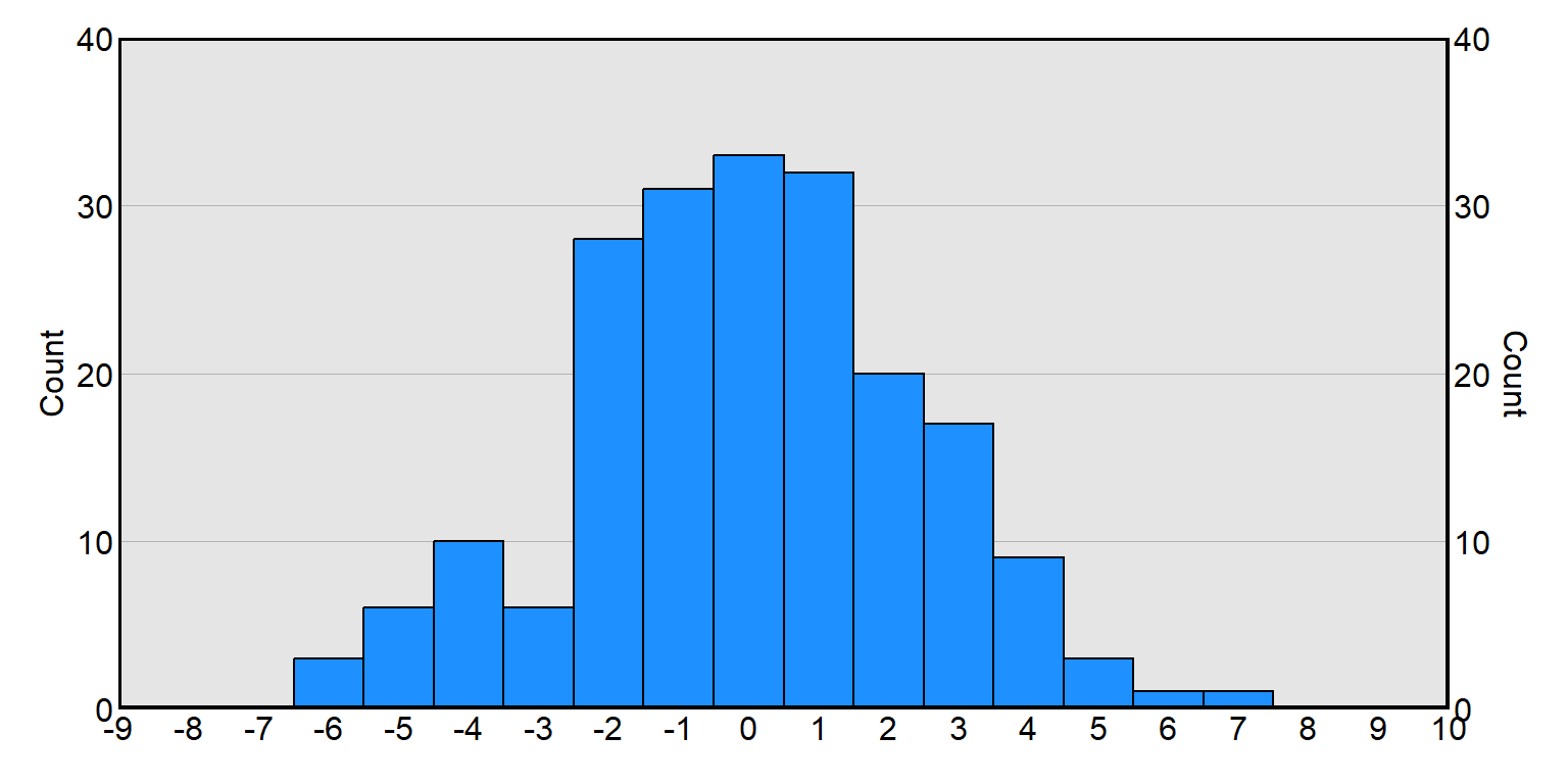
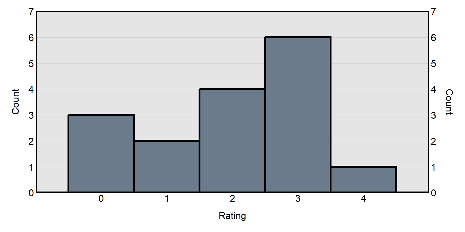
Histograms are plots that indicate how many numbers are at a particular level or fall into into a particular range. The horizontal X-axis of the histogram indicates the level or range, and the vertical Y-axis of the histogram indicates the frequency of how often that level or range occurs in the data.
For example, for the histogram below, there are ten observations of -4 and twenty observations of 2.
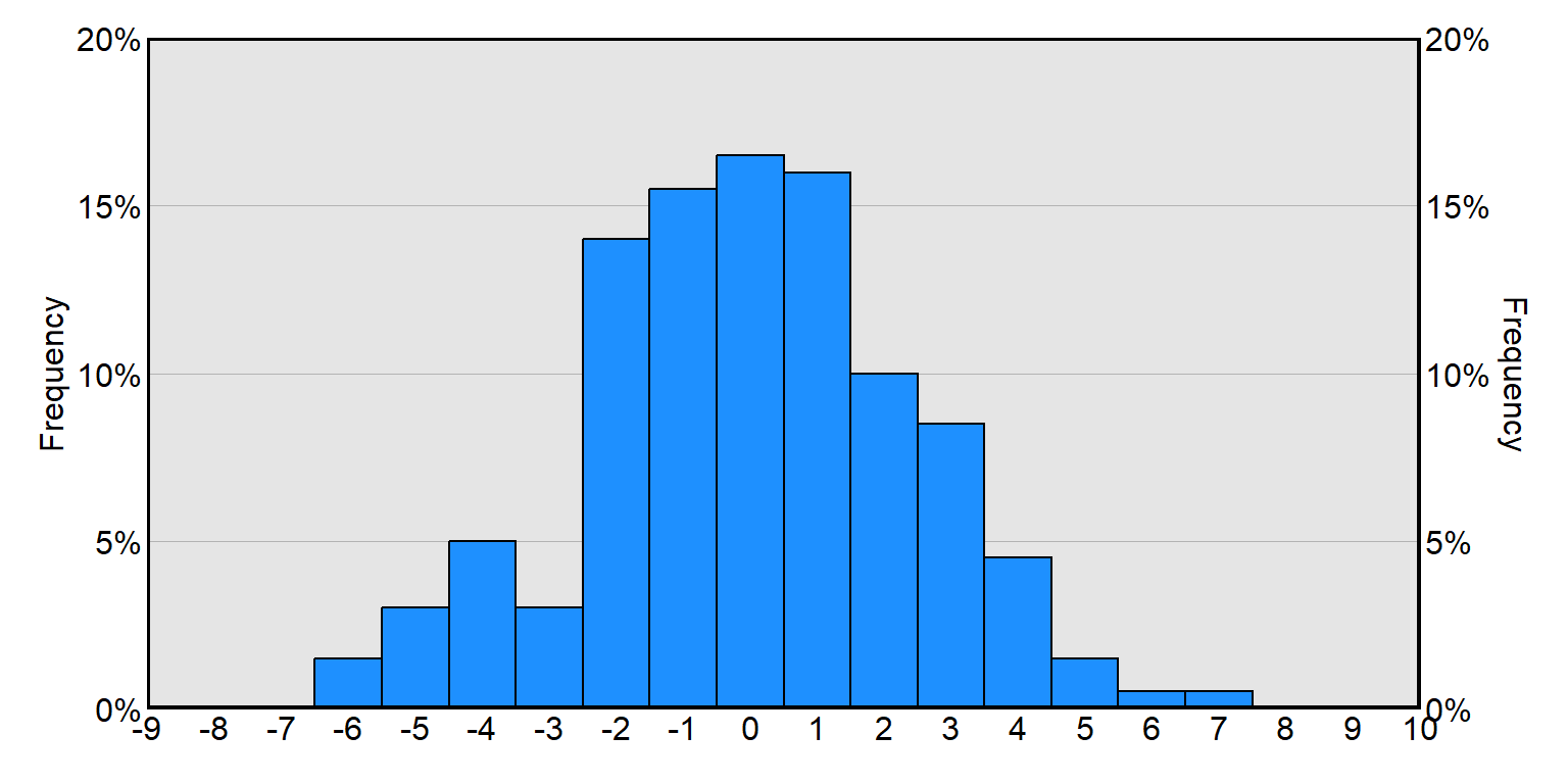
The Y-axis for a histogram can also indicate the percentage of observations that are at each level or fall into each range:
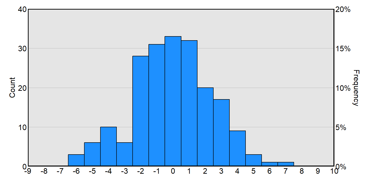
And a histogram can also indicate both counts and percentages:
1.6 Proportions, percentages, and percentage points
Major learning objective(s) for this section:
- Determine a proportion, percentage, percentage change, and percentage point change.
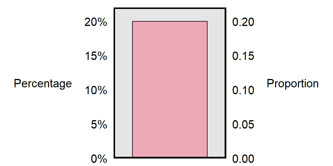
A proportion is a comparison of a part to a whole. Suppose, for example, that a class has 5 female students and 20 male students. The proportion of the class that is female can be expressed as a fraction, in which the numerator (the top number of the fraction) is the number that represents the part that is female (5), and the denominator (the bottom number of the fraction) is the number that represents the whole class (25). The proportion of the class that is female is thus 5 \(\div\) 25 and can be expressed as a decimal as 0.20.
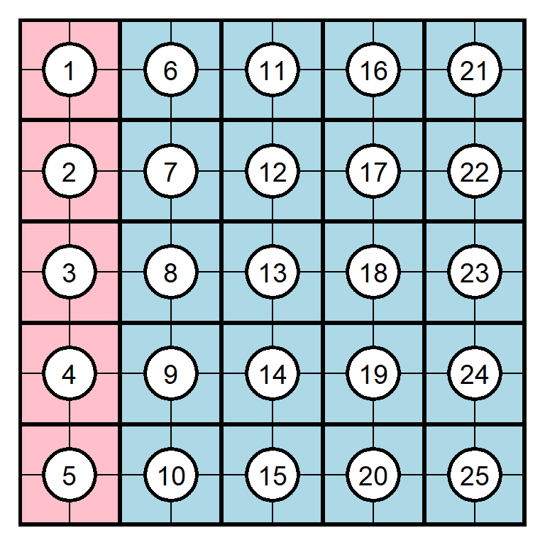
A percentage is the numerator of a proportion when the proportion has a denominator of 100; the “per cent” means “per hundred”. To calculate a percentage, we can multiply the decimal proportion by 100%. So, for a class that has a proportion female of 0.20, the percentage of the class that is female can be calculated as 0.20 \(\times\) 100%, which is 20%.
Suppose that, next year, the class has 15 female students and 35 male students, for a total of 50 students. The proportion of students in that class that is female is now 15 \(\div\) 50 or 0.30, and the percentage of students in that class that is female is now 30%. That change, from 20% female to 30% female, can be expressed in two ways. That change can be expressed as a percentage point change by taking the new percentage and subtracting the old percentage; in this case, that is 30% female minus 20% percent female, to get a change of 10 percentage points. But that change can also be expressed as a percent change, in which the percentage point change is divided by the original percentage:
\[ \frac{\text{10 percentage point change}}{\text{original percentage of 20}} \text{= 0.50 = a 50% change} \]
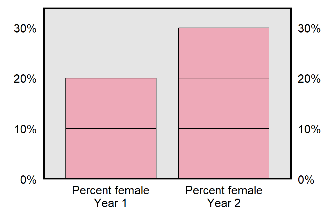
So the same change – from 20% female to 30% female – can be expressed as an increase of 10 percentage points or as an increase of 50 percent. The percentage point description indicates the size of the absolute “raw” difference between the two percentages. The percent description indicates the size of the absolute “raw” difference between the two percentages relative to the starting percentage.
The two types of percentage changes are necessary because there are two ways to think about the size of changes in percentages. Let’s check the data below, for a hypothetical population:
               Year 1   Year 2   pp change   % change
               ----------------  ----------  --------
Republicans      5%       10%       +5pp       100%
Independents    55%       30%
Democrats       40%       60%      +20pp        50%
In a sense, the change in the Democratic percentage was larger than the change in the Republican percentage: the Democratic percentage increased from 40 to 60 (20 percentage points), but the Republican percentage increased only from 5 to 10 (5 percentage points). But, in another sense, the change in the Republican percentage was larger than the change in the Democratic percentage: the Republican percentage doubled (from 5% to 10%), and the Democratic percentage less than doubled (from 40% to 60%).
Sample practice items
Suppose that the percentage of students at a college who are Republican is 20% in 2023 but is 22% in 2024. That change can be correctly expressed as an increase of…
- 2 percentage points
- 10 percentage points
Answer
- 2 percentage points
Suppose that the percentage of students at a college who are Republican is 20% in 2023 but is 22% in 2024. That change can be correctly expressed as an increase of…
- 2%
- 10%
Answer
- 10%
Suppose that the percentage of students at a college who are Democrat is 40% in 2023 but is 50% in 2024. Calculate the percentage point change from 2023 to 2024.
Answer
- 10%
Suppose that the percentage of students at a college who are Democrat is 40% in 2023 but is 50% in 2024. Calculate the percent change from 2023 to 2024.
Answer
- 10%
1.7 Percentiles
Major learning objective(s) for this section:
- Answer items measuring knowledge of the definition of percentile.
This POL 38 course will define percentile so that scoring at the Nth percentile indicates scoring above N% of scores. For example:
- Scoring at the 50th percentile indicates scoring above 50% of scores.
- Scoring at the 95th percentile indicates scoring above 95% of scores.
Imagine, as in the plot below, ten scores arranged from high to low. The lowest score is at the 0th percentile, because that score is above 0 percent of scores. The next higher score is at the 10th percentile, because that score is above 10 percent of scores (above only the lowest score, out of the 10 total scores). The highest score is at the 90th percentile, because that score is above the other 9 of 10 scores.

Percentiles are useful for comparisons: a student getting 90% correct on a test sounds good, but 90% correct might be a relatively low score compared to the student’s peers; in this case, a percentile can be useful for assessing how well a student did relative to the student’s peers.
Remember that percentiles are relative measures: the 50th percentile speed among Olympic sprinters is more impressive than the 50th percentile speed among all persons. The typical Olympic sprinter is on average faster than the typical person, so the middle speed among the set of Olympic sprinters is faster than the middle speed among the set of all persons.
Sample practice items
Suppose that a student scored at the 70th percentile on a test. Which of the following would certainly be true?
- The student got 70% of items correct.
- The student got 70% of items incorrect.
- The student scored better than 70% of test-takers.
- The student scored worse than 70% of test-takers.
Answer
- The student scored better than 70% of test-takers.
The SAT is a test that many high school students take for applying to college. Which is better?
- Scoring at the 1st percentile on the SAT
- Scoring at the 99th percentile on the SAT
Answer
- Scoring at the 99th percentile on the SAT
At the 99th percentile, you score above 99 percent of SAT test-takers, compared to scoring above only 1 percent of SAT test-takers at the 1st percentile.
The SAT is a test that many high school students take for applying to college. The LSAT is a test that many college students take for applying to law school. Which is better, or are both equally impressive achievements?
- Scoring at the 90th percentile on the SAT
- Scoring at the 90th percentile on the LSAT
Answer
- Scoring at the 90th percentile on the LSAT
The LSAT is a more difficult test in which the test-takers are often already in college and are interested in going to law school. Being above 90 percent of these test-takers is more impressive than being above 90 percent of SAT test-takers
Amy and Bob attend different schools. Suppose that Amy and 1,000 other students at her school take a standardized math test, and Amy scores at the 80th percentile on this test among students at her school. Bob and 1,000 different students at his school take the same math test, and Bob scores at the 70th percentile among students at his school. Based on only this information, could we infer that Amy is better in math than Bob is?
- Yes
- No
Answer
- No
No, because the 1,000 students that Amy competed against might be worse in math than the 1,000 students that Bob competed against. Percentile is a relative statistics, and we don’t know the math ability of the students that Amy is compared to relative to the math ability of the students that Bob is compared to.
Suppose that the 16 scores on a test are: 12, 17, 43, 45, 56, 58, 62, 78, 81, 82, 85, 85, 89, 93, 97, and 98. What percentile would the score of 56 be at?
Answer
The score of 56 is above 4 scores, and there are 16 scores, so the score of 56 is above 4/16 or 25% of scores. So 56 is at the 25th percentile.NBA basketball players tend to be taller than the average U.S. resident. Suppose that Bob is at the 80th percentile of height among U.S. residents. Bob’s percentile height among NBA basketball players is likely…
- less than the 80th percentile
- at the 80th percentile
- greater than the 80th percentile
Answer
- less than the 80th percentile
Suppose that a student scored at the 80th percentile on the POL 138 pretest at the start of the semester and then scored at the 50th percentile on the POL 138 posttest at the end of the semester. Which, if any, of the following would necessarily be correct?
- The student got fewer items correct on the posttest than on the pretest.
- The student got a lower percentage of items correct on the posttest than on the pretest.
- The student knew less about the POL 138 material at the end of the semester than the student did at the start of the semester.
- None of the above
Answer
- None of the above
1.8 Weighted means
Major learning objective(s) for this section:
- Determine a weighted mean.
Sometimes, when calculating a mean, it is useful for some observations to get more emphasis (or weight) than other observations get. For example, in school, some courses give more emphasis to particular assessments than to other assessments, such as putting more emphasis on the final exam than on the midterm exam. The general formula for a weighted mean is to take each part of the overall mean, multiply that part by its weight, and then sum all the resulting numbers together.
Suppose, for instance, that a course has a midterm exam that is worth 20% of the final grade and a final exam that is worth 80% of the final grade, and suppose that a student scores 40% on the midterm and 70% on the final exam. We can represent that visually, as in the plot below:
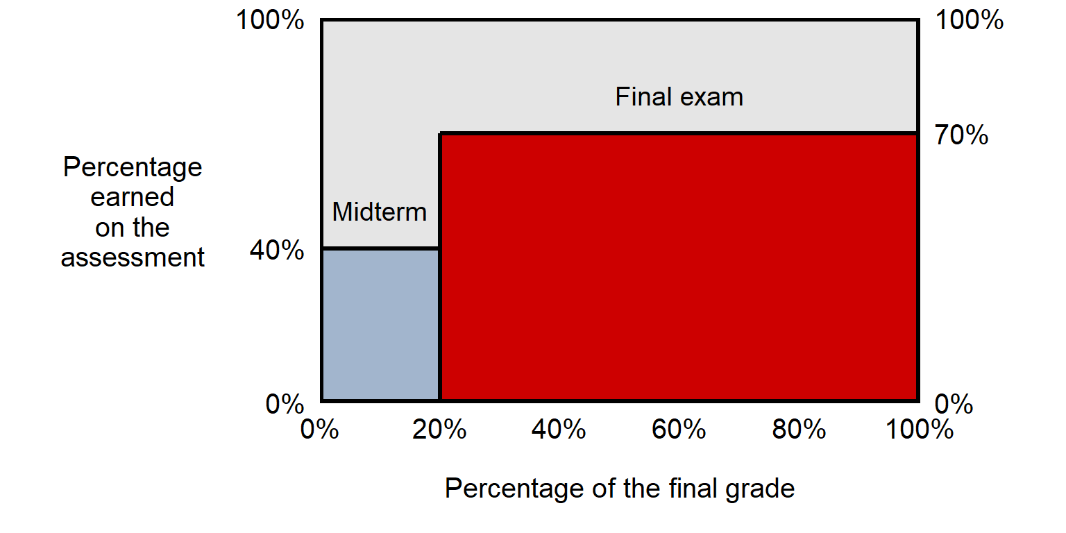
We can calculate the student’s final grade accounting for the fact that the final exam gets more weight than the midterm, by calculating the areas for each part of the final grade and them adding the areas together, as follows:
(Midterm score)×(Midterm weight) + (Final exam score)×(Final exam weight)
          (40%)×(0.20)           +              (70%)×(0.80)
               8%                +                  56%
                                64%
Note that it doesn’t matter whether you multiply the score by the weight (in that order) or multiply the weight by the score (in that order).
For the plot, the 64% weighted mean represents the fact that the student’s performance covered 64 percent of the area, in which the midterm exam counts 20% toward the total and the final exam counts 80% toward the total.
Another way to think about the prior problem is that the final exam – at 80% of the final grade – is worth four times as much as the midterm exam at 20% of the final grade. Thus, we can imagine that there are four times as many final exam scores as there are midterm exam scores, such as:
40% 70% 70% 70% 70%
If we sum those 5 grades and then divide by the number of grades, we get:
40% + 70% + 70% + 70% + 70%
320% / 5
64%
Sample practice items
Let’s imagine a similar situation to the above situation, but in which the midterm score and the final exam score are reversed. Calculate the weighted mean for a situation in which the midterm counts for 20% of the final grade, the final exam counts for 80% of the final grade, the student scored 70% on the midterm, and the student scored 40% on the final exam.
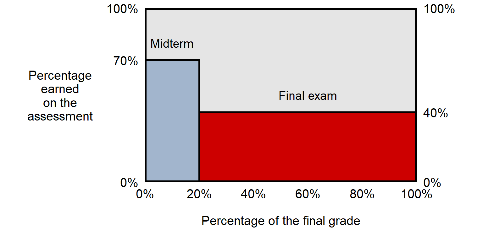
Answer
(70%)×(0.20) + (40%)×(0.80) =
    14%      + 32%          =
            46%
Suppose that a course has three exams: Exam 1 (worth 20% of the overall grade for the course), Exam 2 (worth 30% of the overall grade for the course), and a Final Exam (worth 50% of the overall grade for the course). A student scored 90% on Exam 1, 80% on Exam 2, and 70% on the Final Exam. What is the student’s overall grade for the course?
Answer
(90%)×(0.20) + (80%)×(0.30) + (70%)×(0.50) =
    18%      +     24%      + 35%          =
                   77%
Extra practice item
Suppose that, in a POL 138 course, a student has scored 88% on everything except for the final exam. The final exam is worth 20% of the final grade. This course has no bonus. To the nearest whole percentage, what must the student’s percentage be on the final exam so that the student’s final grade is 90%?
Answer
This involves a bit of algebra, in which we can use X to represent the unknown final exam percentage:
(88)×(0.80) + X(0.20) =  90
   70.4     +  0.20X  =  90
  -70.4                 -70.4 [subtract 70.4 from both sides of the equals sign]
           0.20X      =  19.6
            X         =  98
1.9 Probability
Major learning objective(s) for this section:
- Correctly apply the product rule for probability.
- Correctly identify when the product rule should not be applied.
For a set of outcomes that are equally likely, the probability of a particular outcome can be calculated as:
\[\small\text{Probability of an outcome}=\frac{\text{Number of times the outcome occurs}}{\text{Number of equally-likely outcomes that can occur}}\]
Let’s consider a fair coin, in which one side is heads and the other side is tails, and in which the probability that the coin lands on heads equals the probability that the coin lands on tails. If we flip a fair coin once, there are two possible outcomes – heads and tails – and both outcomes are equally likely. We can thus correctly state that the probability of getting heads on a flip of a fair coin is 1 of 2 (or 50%), because there are 2 possible outcomes (so the denominator is 2) and we are interested in the probability that one of these outcomes occur (a heads).
Suppose that we flip a fair coin twice. There are four possible outcomes, each of which is equally likely:
HH HT TH TT
We can thus correctly state that the probability of getting least one heads on two flips of a fair coin is 3 of 4 (or 75%), because there are 4 possible outcomes (so the denominator is 4) and we are interested in three of these outcomes (HH, HT, and TH, because these are the outcomes with at least one heads). Moreover, we can correctly state that the probability of getting heads twice (HH) on two flips of a fair coin is 1 of 4 (or 25%).
Suppose that we flip a fair coin three times. There are now eight possible outcomes, each of which is equally likely:
HHH HHT HTT TTT
    HTH THT
    THH TTH
We can thus state correctly that the probability of getting heads three times (HHH) on three flips of a fair coin is \(1\div8\) (or 12.5%).
Product rule
Suppose that we wanted to calculate the probability of getting five heads in five flips of a fair coin. Instead of writing out all possible outcomes for five flips of a fair coin, we can use a shortcut called the product rule. The product rule is that, if the probability that A occurs does not influence the probability that B occurs (in other words, if A and B are independent events), then the probability that both A and B occur can be calculated using multiplication:
Probability that A and B both occur =
  the probability that A occurs ×
    the probability that B occurs
This can be extended to more than two independent events. For example, if probability of the three outcomes A, B, and C are all independent of each other, then the probability that all three occur is:
Probability that A, B, and C all occur =
  the probability that A occurs ×
    the probability that B occurs ×
      the probability that C occurs
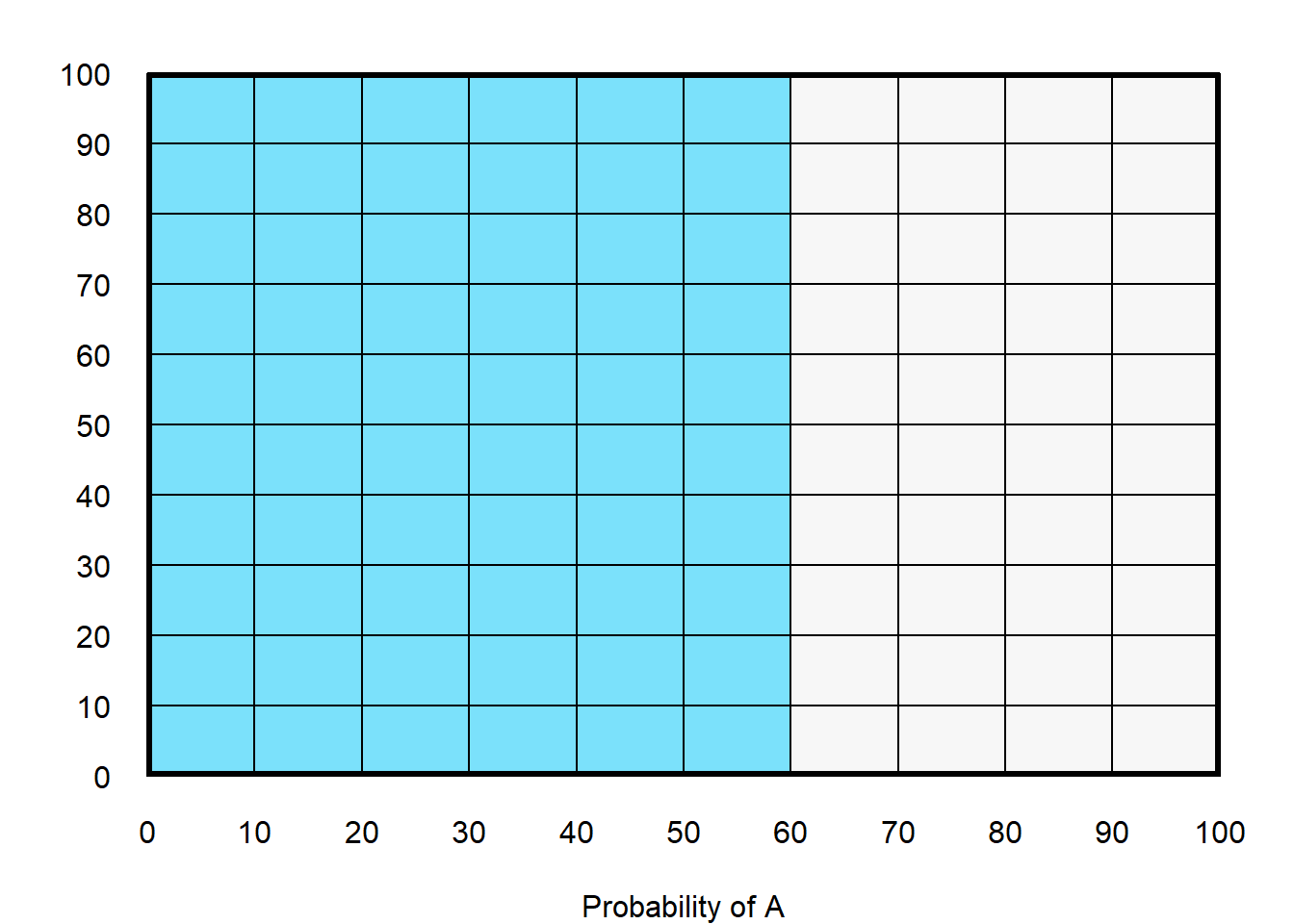
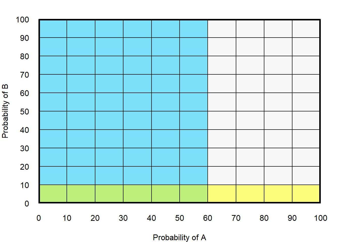
Below is an illustration of the product rule for two outcomes A and B. In the plot below, the vertical blue shaded area represents a 60% probability that A occurs (shaded from A=0 to A=60, on an axis in which A ranges from 0 to 100).
In the plot below, the horizontal yellow shaded area represents a 10% probability that B occurs (shaded from B=0 to B=10, on an axis in which B ranges from 0 to 100).
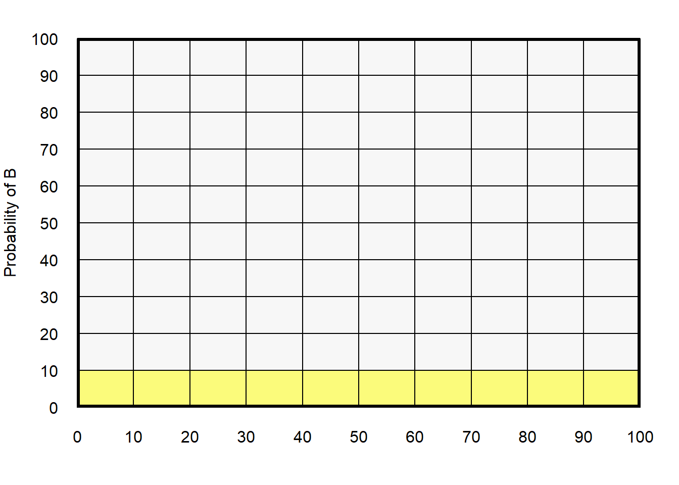
In the plot below, the “double shaded” blue/yellow area represents the probability that both A and B occur. The “double shaded” blue/yellow area is 6% of the total area (with purple cells being 6 of the 100 total cells).
Non-independent events
The product rule cannot be properly applied when probabilities are not independent of each other.
For example, suppose that 60% of students at a university are female and that 10% of students at that university are in a nursing program. The probability is 60% that a randomly selected student is female, and the probability is 10% that a randomly selected student is in the nursing program, but we cannot properly conclude that the probability that a randomly selected student is a female nursing student is \(60\%\times10\% = 6\%\), because the probability of being female might not be independent of the probability of being in the nursing program. See the table below, in which 60% of students are female and 10% of students at the university are in a nursing program, but the probability is 9% (9 of 100) that a randomly selected student is female and in the nursing program.
| Female | Male | TOTAL | |
|---|---|---|---|
| In the nursing program | 9 | 1 | 10 |
| Not in the nursing program | 51 | 39 | 90 |
| TOTAL | 60 | 40 | 100 |
The product rule did not work in this case because the probability of being female was not independent of the probability of being in the nursing program, in that females are a higher percentage of nursing students than of other students.
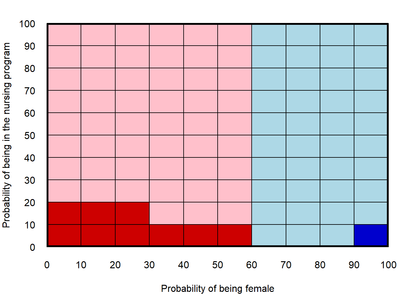
The plot below illustrates why the product rule did not work in this case. The dark red and light red regions indicate the 60% probability of being female, and the dark blue and light blue regions indicate the 40% probability of being male. The dark regions represent students in the nursing program, but the probability of being in the nursing program is not independent of the probability of being female: 15% of female students are in the nursing program (9 of 60), but only 2.5% of male students are in the nursing program (1 of 40), so the dark shaded area is disjointed.
Product rule without replacement
Let’s consider a standard deck of cards that has 4 aces among the 52 cards. Suppose that we draw one card from the deck, put that card back in the deck, and then draw another card from the deck. The probability that we drew an ace both times is:
(4 ÷ 52) × (4 ÷ 52) =
16 ÷ 2704 =
0.59%
The above example can be referred to as drawing cards “with replacement”, because the cards that we drew were placed back into the deck before we drew again. But we can also draw cards without replacement, by keeping the cards that we drew out of the deck so that there are fewer cards when we draw again…
Let’s imagine that we draw 4 cards without replacement, so that we are holding 4 cards and there are 48 cards that we are not holding. Let’s calculate the probability that all four of our cards are aces. The probability that the first card drawn is an ace is \(4\div52\), because there are 52 total cards and, of these 52 cards, only 4 are aces. But to calculate the probability that the second card is an ace, we need to account for the fact that, if we draw an ace on the first card, there are fewer than four aces remaining and fewer than 52 cards remaining. So the probability that the second card drawn is an ace is \(3\div51\), because – after we drew an ace on the first card – the deck of cards has 3 aces remaining out of 51 cards remaining. And the probability that the third card drawn is an ace is \(2\div50\). And the probability that the fourth card drawn is an ace is \(1\div49\). So the probability that all four of our cards are aces is:
(4 ÷ 52) × (3 ÷ 51) × (2 ÷ 50) × (1 ÷ 49) =
24 ÷ 6497400 =
0.00037%
Sample practice items
The probability of X happening is 20%, and the probability of Y happening is 10%. X and Y are independent events. What is the probability that X and Y both occur?
- 0.20 + 0.10
- 0.20 \(\times\) 0.10
- 0.20 \(\div\) 0.10
- (0.20 + 0.10) \(\div\) 2
- Cannot be determined from the information provided
Answer
- 0.20 \(\times\) 0.10
The probability of X happening is 20%, and the probability of Y happening is 10%. X and Y are not independent events. What is the probability that X and Y both occur?
- 0.20 + 0.10
- 0.20 \(\times\) 0.10
- 0.20 \(\div\) 0.10
- (0.20 + 0.10) \(\div\) 2
- Cannot be determined from the information provided
Answer
- Cannot be determined from the information provided
The probability of getting heads on each flip of a fair coin is 50%, and one flip of the coin does not influence another flip of the coin. Using the product rule, what is the probability of flipping a fair coin twice and getting two heads?
- 0.50 + 0.50
- 0.50 \(\times\) 0.50
- The product rule should not be used for this item.
Answer
- 0.50 \(\times\) 0.50
The probability of getting heads on each flip of a fair coin is 50%, and one flip of the coin does not influence another flip of the coin. Using the product rule, what is the probability of flipping a fair coin exactly four times and getting exactly four heads?
Answer
(0.50) \(\times\) (0.50) \(\times\) (0.50) \(\times\) (0.50) = 0.0625 = 6.25%Suppose that you flip a fair coin one thousand times. Is it possible that all of the flips land on heads?
- Yes
- No
Answer
- Yes
Suppose that a particular defendant is on trial and that, in the population, 95 percent of persons would vote to convict this defendant based on the evidence presented at trial. Suppose that 12 persons are randomly drawn from the population to serve on a jury for this defendant. To the nearest whole number percentage, what is the probability that all 12 of these jurors will vote to convict the defendant based on the evidence presented at trial, assuming that no juror influences the vote of any other juror?
Answer
(0.95)12 = 54%Suppose that, in a given population, 40% of persons are men, and 60% of persons are women. Suppose also that, in this population, 40% of persons are Democrats, 22% of persons are Independents, and 38% of persons are Republicans. Suppose that we want to calculate the probability that a given person randomly drawn from this population is a woman Democrat. Explain why we cannot use the product rule to calculate that probability as being \(0.60\times0.40\), to get a 24% probability that that randomly drawn person is a woman Democrat.
Answer
The product rule cannot be used in this situation because the probability of being a woman might not be independent of the probability of being a Democrat. For example, in the United States, women are currently more likely to identify as Democrat than as Republican, and men are currently more likely to identify as Republican than as Democrat.
Suppose that 50% of a population is female and that 60% of the population attends religious services. Discuss whether we can use the product rule to validly estimate that about 30% of the population are females who attend religious services.
Answer
The product rule should not be used for this item, because we do not know the relationship between gender and attending religious services. In the United States, for example, women have been more likely to report attending religious services than men have been, so the probability of being female might not be independent of the probability of attending religious services.Suppose that we have 26 red cards and 26 black cards, for a total of 52 cards. We draw three cards, so that we are holding three cards, and there are 49 cards that we are not holding. Calculate the probability that all three of our cards are red cards.
Answer
The probability that the first card drawn is red is \(26\div52\). But once a red card is drawn, there are fewer red cards remaining and fewer cards remaining. The probability that the second card drawn is red is thus \(25\div51\). And the probability that the third card drawn is red is \(24\div50\). So the probability that all three of our cards are red cards is:(26 ÷ 52) × (25 ÷ 51) × (24 ÷ 50) = 15600 ÷ 132600 = 0.12, which is about 12%