Below are leftover comments on publications that I read in 2021.

---

ONO AND ZILIS 2021

Politics, Groups, and Identities published Ono and Zilis 2021, "Do Americans perceive diverse judges as inherently biased?". Ono and Zilis 2021 indicated that "We test whether Americans perceive diverse judges as inherently biased with a list experiment". The statements to test whether Americans perceive diverse judges to be "inherently biased" were:

When a court case concerns issues like #metoo, some women judges might give biased rulings.

When a court case concerns issues like immigration, some Hispanic judges might give biased rulings.

Ono and Zilis 2021 indicated that "...by endorsing that idea, without evidence, that 'some' members of a group are inclined to behave in an undesirable way, respondents are engaging in stereotyping" (pp. 3-4).

But statements about whether *some* Hispanic judges and *some* women judges *might* be biased can't measure stereotypes or the belief that Hispanic judges or women judges are *inherently* biased. For example, a belief that *some* women *might* commit violence doesn't require the belief that women are inherently violent and doesn't even require the belief that women are on average more violent than men are.

---

Ono and Zilis 2021 claimed that "Hispanics do not believe that Hispanic judges are biased" (p. 4, emphasis in the original), but, among Hispanic respondents, the 95% confidence interval for agreement with the claim that Hispanic judges might be biased in cases involving issues like immigration did not cross zero in the multivariate analyses in Figure 1.

For Table 2 analyses without controls, the corresponding point estimate indicated that 25 percent of Hispanics agreed with the claim about Hispanic judges, but the ratio of the relevant coefficient to standard error was 0.25/0.15, which is about 1.67, depending on how the 0.25 and 0.15 were rounded. The corresponding p-value isn't less than p=0.05, but that doesn't support the conclusion that the percentage of Hispanics that agreed with the statement is zero.

---

BERRY ET AL 2021

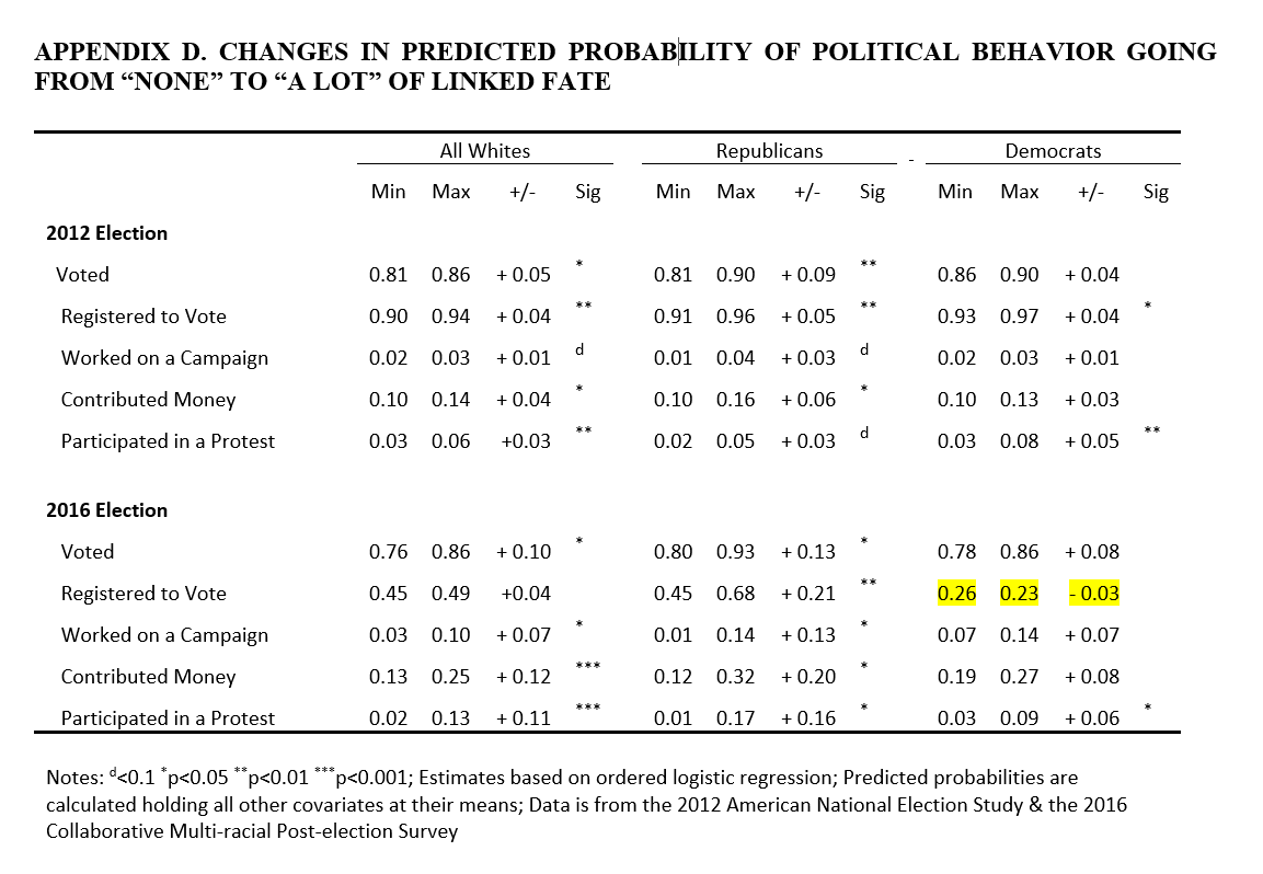
Politics, Groups, and Identities published Berry et al 2021,"White identity politics: linked fate and political participation". Berry et al 2021 claimed to have found "notable partisan differences in the relationship between racial linked fate and electoral participation for White Americans". But this claim is based on differences in the presence of statistical significance between estimates for White Republicans and estimates for White Democrats ("Linked fate is significantly and consistently associated with increased electoral participation for Republicans, but not Democrats", p. 528), instead of being based on statistical tests of whether estimates for White Republicans differ from estimates for White Democrats.

The estimates in the Berry et al 2021 appendix that I highlighted in yellow appear to be incorrect, in terms of plausibility and based on the positive estimate in the corresponding regression output.

---

ARCHER AND CLIFFORD FORTHCOMING

In "Improving the Measurement of Hostile Sexism" (reportedly forthcoming at Public Opinion Quarterly), Archer and Clifford proposed a modified version of the hostile sexism scale that is item specific. For example, instead of measuring responses about the statement "Women exaggerate problems they have at work", the corresponding item-specific item measures responses to the question of "How often do women exaggerate problems they have at work?". Thus, to get the lowest score on the hostile sexism scale, instead of merely strongly disagreeing that women exaggerate problems they have at work, respondents must report the belief that women *never* exaggerate problems they have at work.

---

Archer and Clifford indicated that responses to some of their revised items are measured on a bipolar scale. For example, respondents can indicate that women are offended "much too often", "a bit too often", "about the right amount", "not quite often enough", or "not nearly often enough". So to get the lowest hostile sexism score, respondents need to indicate that women are wrong about how often they are offended, by not being offended enough.

Scott Clifford, co-author of the Archer and Clifford article, engaged me in a discussion about the item specific scale (archived here). Scott suggested that the low end of the scale is more feminist, but dropped out of the conversation after I asked how much of an OLS coefficient for the proposed item-specific hostile sexism scale is due to hostile sexism and how much is due to feminism.

The portion of the hostile sexism measure that is sexism seems like something that should have been addressed in peer review, if the purpose of a hostile sexism scale is to estimate the effect of sexism and not to merely estimate the effect of moving from highly positive attitudes about women to highly negative attitudes about women.

---

VIDAL ET AL 2021

Social Science Quarterly published Vidal et al,"Identity and the racialized politics of violence in gun regulation policy preferences". Appendix A indicates that, for the American National Election Studies 2016 Time Series Study, responses to the feeling thermometer about Black Lives Matter ranged from 0 to 999, with a standard deviation of 89.34, even though the ANES 2016 feeling thermometer for Black Lives Matter ran from 0 to 100, with 999 reserved for respondents who indicate that they don't know what Black Lives Matter is.

---

ARORA AND STOUT 2021

Research & Politics published Arora and Stout 2021 "After the ballot box: How explicit racist appeals damage constituents views of their representation in government", which noted that:

The results provide evidence for our hypothesis that exposure to an explicitly racist comment will decrease perceptions of interest representation among Black and liberal White respondents, but not among moderate and conservative Whites.

This is, as far as I can tell, a claim that the effect among Black and liberal White respondents will differ from the effect among moderate and conservative Whites, but Arora and Stout 2021 did not report a test of whether these effects differ, although Arora and Stout 2021 did discuss statistical significance for each of the four groups.

Moreover, Arora and Stout 2021 footnote 4 indicates that:

In the supplemental appendix, we confirm that explicit racial appeals have a unique effect on interest representation and are not tied to other candidate evaluations such as vote choice.

But the estimated effect for interest representation (Table 1) was -0.06 units among liberal White respondents (with a "+" indicator for statistical significance), which is the same reported number as the estimated effect for vote choice (Table A5): -0.06 units among liberal White respondents (with a "+" indicator for statistical significance).

None of the other estimates in Table 1 or Table A5 have an indicator for statistical significance.

---

Arora and Stout 2021 repeatedly labeled as "explicitly racist" the statement that "If he invited me to a public hanging, I'd be on the front row", but it's not clear to me how that statement is explicitly racist. The Data and Methodology section indicates that "Though the comment does not explicitly mention the targeted group...". Moreover, the Conclusion of Arora and Stout 2021 indicates that...

In spite of Cindy Hyde-Smith's racist comments during the 2018 U.S. Senate election which appeared to show support for Mississippi's racist and violent history, she still prevailed in her bid for elected office.

... and "appeared to" isn't language that I would expect from an explicit statement.

---

CHRISTIANI ET AL 2021

The Journal of Race, Ethnicity, and Politics published Christiani et al 2021 "Masks and racial stereotypes in a pandemic: The case for surgical masks". The abstract indicates that:

...We find that non-black respondents perceive a black male model as more threatening and less trustworthy when he is wearing a bandana or a cloth mask than when he is not wearing his face covering—especially those respondents who score above average in racial resentment, a common measure of racial bias. When he is wearing a surgical mask, however, they do not perceive him as more threatening or less trustworthy. Further, it is not that non-black respondents find bandana and cloth masks problematic in general. In fact, the white model in our study is perceived more positively when he is wearing all types of face coverings.

Those are the within-model patterns, but it's interesting to compare ratings of the models in the control, pictured below:

Appendix Table B.1 indicates that, on average, non-Black respondents rated the White model more threatening and more untrustworthy compared to the Black model: on a 0-to-1 scale, among non-Black respondents, the mean ratings of "threatening" were 0.159 for the Black model and 0.371 for the White model, and the mean ratings of "untrustworthy" were 0.128 for the Black model and 0.278 for the White model. These Black/White gaps were about five times the standard errors.

Christiani et al 2021 claimed that this baseline difference does not undermine their results:

Fortunately, the divergent evaluations of our two models without their masks on do not undermine either of the main thrusts of our analyses. First, we can still compare whether subjects perceive the black model differently depending on what type of mask he is wearing...Second, we can still assess whether people resolve the ambiguity associated with seeing a man in a mask based on the race of the wearer.

But I'm not sure that it is true, that "divergent evaluations of our two models without their masks on do not undermine either of the main thrusts of our analyses".

I tweeted a question to one of the Christiani et al 2021 co-authors that included the handles of two other co-authors, asking whether it was plausible that masks increase the perceived threat of persons who look relatively nonthreatening without a mask but decrease the perceived threat of persons who look relatively more threatening without a mask. That phenomenon would explain the racial difference in patterns described in the abstract, given that the White model in the control was perceived to be more threatening than the Black model in the control.

No co-author has yet responded to defend their claim.

---

Below are the mean ratings on the 0-to-1 "threatening" scale for models in the "no mask" control group, among non-Black respondents by high and low racial resentment, based on Tables B.2 and B.3:

Non-Black respondents with high racial resentment
0.331 mean "threatening" rating of the White model
0.376 mean "threatening" rating of the Black model

Non-Black respondents with low racial resentment
0.460 mean "threatening" rating of the White model
0.159 mean "threatening" rating of the Black model

---

VICUÑA AND PÉREZ 2021

Politics, Groups, and Identities published Vicuña and Pérez 2021, "New label, different identity? Three experiments on the uniqueness of Latinx", which claimed that:

Proponents have asserted, with sparse empirical evidence, that Latinx entails greater gender-inclusivity than Latino and Hispanic. Our results suggest this inclusivity is real, as Latinx causes individuals to become more supportive of pro-LGBTQ policies.

The three studies discussed in Vicuña and Pérez 2021 had these prompts, with the bold font in square brackets indicating the differences in treatments across the four conditions:

Using the spaces below, please write down three (3) attributes that make you [a unique person/Latinx/Latino/Hispanic]. These could be physical features, cultural practices, and/or political ideas that you hold [as a member of this group].

If the purpose is to assess whether "Latinx" differs from "Latino" and "Hispanic", I'm not sure of the value of the "a unique person" treatment.

Discussing their first study, Vicuña and Pérez 2021 reported the p-value for the effect of the "Latinx" treatment relative to the "unique person" treatment (p<.252) and reported the p-values for the effect of the "Latinx" treatment relative to the "Latino" treatment (p<.046) and the "Hispanic" treatment (p<.119). Vicuña and Pérez 2021 reported all three corresponding p-values when discussing their second study and their third study.

But, discussing their meta-analysis of the three studies, Vicuña and Pérez 2021 reported one p-value, which is presumably for the effect of the "Latinx" treatment relative to the "unique person" treatment.

I tweeted a request Dec 20 to the authors to post their data, but I haven't received a reply yet.

---

KIM AND PATTERSON JR. 2021

Political Science & Politics published Kim and Patterson Jr. 2021, "The Pandemic and Gender Inequality in Academia", which reported on tweets of tenure-track political scientists in the United States.

Kim and Patterson Jr. 2021 Figure 2 indicates that, in February 2020, the percentage of work-related tweets was about 11 percent for men and 11 percent for women, and that, shortly after Trump declared a national emergency, these percentages had dropped to about 8 percent and 7 percent respectively. Table 2 reports difference-in-difference results indicating that the pandemic-related decrease in the percentage of work-related tweets was 1.355 percentage points larger for women than for men.

That seems like a relatively small gender inequality in size and importance, and I'm not sure that this gender inequality in percentage of work-related tweets offsets the advantage of having the 31.5k follower @womenalsoknow account tweet about one's research.

---

The abstract of Kim and Patterson Jr. 2021 refers to "tweets from approximately 3,000 political scientists". Table B1 in Appendix B has sample size of 2,912, with a larger number of women than men at the rank of assistant professor, at the rank of associate professor, and at the rank of full professor. The APSA dashboard indicates that women were 37% of members of the American Political Science Association and that 79.5% of APSA members are in the United States, so I think that Table B1 suggests that a higher percentage of female political scientists might be on Twitter than male political scientists.

Oddly, though, when discussing the representatives of this sample, Kim and Patterson Jr. 2021 indicated that (p. 3):

Yet, relevant to our design, we found no evidence that female academics are less likely to use Twitter than male colleagues conditional on academic rank.

That's true about not being *less* likely, but my analysis of the data for Kim and Patterson Jr. 2021 Table 1 indicated that, controlling for academic rank, about 5 percent more female political scientists from top 50 departments were on Twitter, compared to male political scientists from top 50 departments.

Table 1 of Kim and Patterson Jr. 2021 is limited to the 1,747 tenure-track political scientists in the United States from top 50 departments. I'm not sure why Kim and Patterson Jr. 2021 didn't use the full N=2,912 sample for the Table 1 analysis.

---

My analysis indicated that the female/male gaps in the sample were as follows: 2.3 percentage points (p=0.655) among assistant professors, 4.5 percentage points (p=0.341) among associate professors, and 6.7 percentage points (p=0.066) among full professors, with an overall 5 percentage point male/female gap (p=0.048) conditional on academic rank.

---

Kim and Patterson Jr. 2021 suggest a difference in the effect by rank:

Disaggregating these results by academic rank reveals an effect most pronounced among assistants, with significant—albeit smaller—effects for associates. There is no differential effect on work-from-home at the rank of full professor, which is consistent with our hypothesis that these gaps are driven by the increased obligations placed on women who are parenting young children.

But I don't see a test for whether the coefficients differ from each other. For example, in Table 2 for work-related tweets, the "Female * Pandemic" coefficient is -1.188 for associate professors and is -0.891 for full professors, for a difference of 0.297, relative to the respective standard errors of 0.579 and 0.630.

---

Table 1 of Kim and Patterson Jr. 2021 reported a regression predicting whether a political scientist in a top 50 department was a Twitter user, and the p-values are above p=0.05 for all coefficients for "female" and for all interactions involving "female". That might be interpreted as a lack of evidence for a gender difference in Twitter use among these political scientists, but the interaction terms don't permit a clear inference about an overall gender difference.

For example, associate professor is the omitted category of rank in the regression, so the 0.045 non-statistically significant "female" coefficient indicates only that female associate professor political scientists from top 50 departments were 4.5 percentage points more likely to be a Twitter user than male associate professor political scientists from top 50 departments.

And the non-statistically significant "Female X Assistant" coefficient doesn't indicate whether female assistant professors differ from male assistant professors: instead, the non-statistically significant "Female X Assistant" coefficient indicates only that the associate/assistant difference among men in the sample does not differ at p<0.05 from the associate/assistant difference among women in the sample.

Link to the data. R code for my analysis. R output from my analysis.

---

LEFTOVER PLOT

I had the plot below for a draft post that I hadn't yet published:

Item text: "For each of the following groups, how much discrimination is there in the United States today?" [Blacks/Hispanics/Asians/Whites]. Substantive response options were: A great deal, A lot, A moderate amount, A little, and None at all.

Data source: American National Election Studies. 2021. ANES 2020 Time Series Study Preliminary Release: Combined Pre-Election and Post-Election Data [dataset and documentation]. March 24, 2021 version. www.electionstudies.org.

Stata and R code. Dataset for the plot.

Tagged with: , , , ,

I had a recent Twitter exchange about a Monkey Cage post:

Below, I use statistical power calculations to explain why the Ahlquist et al. paper, or at least the list experiment analysis cited in the Monkey Cage post, is not compelling.

---

Discussing the paper (published version here), Henry Farrell wrote:

So in short, this research provides exactly as much evidence supporting the claim that millions of people are being kidnapped by space aliens to conduct personally invasive experiments on, as it does to support Trump's claim that millions of people are engaging in voter fraud.

However, a survey with a sample size of three would also not be able to differentiate the percentage of U.S. residents who commit vote fraud from the percentage of U.S. residents abducted by aliens. For studies that produce a null result, it is necessary to assess the ability of the study to detect an effect of a particular size, to get a sense of how informative that null result is.

The Ahlquist et al. paper has a footnote [31] that can be used to estimate the statistical power for their list experiments: more than 260,000 total participants would be needed for a list experiment to have 80% power to detect a 1 percentage point difference between treatment and control groups, using an alpha of 0.05. The power calculator here indicates that the corresponding estimated standard deviation is at least 0.91 [see note 1 below].

So let's assume that list experiment participants are truthful and that we combine the 1,000 participants from the first Ahlquist et al. list experiment with the 3,000 participants from the second Ahlquist et al. list experiment, so that we'd have 2,000 participants in the control sample and 2,000 participants in the treatment sample. Statistical power calculations using an alpha of 0.05 and a standard deviation of 0.91 indicate that there is:

  • a 5 percent chance of detecting a 1% rate of vote fraud.
  • an 18 percent chance of detecting a 3% rate of vote fraud.
  • a 41 percent chance of detecting a 5% rate of vote fraud.
  • a 79 percent chance of detecting an 8% rate of vote fraud.
  • a 94 percent chance of detecting a 10% rate of vote fraud.

---

Let's return to the claim that millions of U.S. residents committed vote fraud and use 5 million for the number of adult U.S. residents who committed vote fraud in the 2016 election, eliding the difference between illegal votes and illegal voters. There are roughly 234 million adult U.S. residents (reference), so 5 million vote fraudsters would be 2.1% of the adult population, and a 4,000-participant list experiment would have about an 11 percent chance of detecting that 2.1% rate of vote fraud.

Therefore, if 5 million adult U.S. residents really did commit vote fraud, a list experiment with the sample size of the pooled Ahlquist et al. 2014 list experiments would produce a statistically-significant detection of vote fraud about 1 of every 9 times the list experiment was conducted. The fact that Ahlquist et al. 2014 didn't detect voter impersonation at a statistically-significant level doesn't appear to compel any particular belief about whether the rate of voter impersonation in the United States is large enough to influence the outcome of presidential elections.

---

NOTES

1. Enter 0.00 for mu1, 0.01 for mu2, 0.91 for sigma, 0.05 for alpha, and a 130,000 sample size for each sample; then hit Calculate. The power will be 0.80.

2. I previously discussed the Ahlquist et al. list experiments here and here. The second link indicates that an Ahlquist et al. 2014 list experiment did detect evidence of attempted vote buying.

Tagged with: , , ,

Researchers often have the flexibility to report only the results they want to report, so an important role for peer reviewers is to request that researchers report results that a reasonable skeptical reader might suspect have been strategically unreported. I'll discuss two publications where obvious peer review requests do not appear to have been made and, presuming these requests were not made, how requests might have helped readers better assess evidence in the publication.

---

Example 1. Ahlquist et al. 2014 "Alien Abduction and Voter Impersonation in the 2012 U.S. General Election: Evidence from a Survey List Experiment"

Ahlquist et al. 2014 reports on two list experiments: one list experiment is from December 2012 and has 1,000 cases, and another list experiment is from September 2013 and has 3,000 cases.

Figure 1 of Ahlquist et al. 2014 reports results for the 1,000-person list experiment estimating the prevalence of voter impersonation in the 2012 U.S. general election; the 95% confidence intervals for the full sample and for each reported subgroup cross zero. Figure 2 reports results for the full sample of the 3,000-person list experiment estimating the prevalence of voter impersonation in the 2012 U.S. general election, but Figure 2 did not include subgroup results. Readers are thus left to wonder why subgroup results were not reported for the larger sample that had more power to detect an effect among subgroups.

Moreover, the main voting irregularity list experiment reported in Ahlquist et al. 2014 concerned voter impersonation, but, in footnote 15, Ahlquist et al. discuss another voting irregularity list experiment that was part of the study, about whether political candidates or activists offered the participant money or a gift for their vote:

The other list experiment focused on vote buying and closely mimicked that described in Gonzalez-Ocantos et al. (2012). Although we did not anticipate discovering much vote buying in the USA we included this question as a check, since a similar question successfully discovered voting irregularities in Nicaragua. As expected we found no evidence of vote buying in the USA. We omit details here for space considerations, though results are available from the authors and in the online replication materials...

The phrasing of the footnote is not clear whether the inference of "no evidence of vote buying in the USA" is restricted to an analysis of the full sample or also covers analyses of subgroups.

So the article leaves at least two questions unanswered for a skeptical reader:

  1. Why report subgroup analyses for only the smaller sample?
  2. Why not report the overall estimate and subgroup analyses for the vote buying list experiment?

Sure, for question 2, Ahlquist et al. indicate that the details of the vote buying list experiment were omitted for "space considerations"; however, the 16-page Ahlquist et al. 2014 article is shorter than the other two articles in the journal issue, which are 17 pages and 24 pages.

Peer reviewer requests that could have helped readers were to request a detailed report on the vote buying list experiment and to request a report of subgroup analyses for the 3,000-person sample.

---

Example 2. Sen 2014 "How Judicial Qualification Ratings May Disadvantage Minority and Female Candidates"

Sen 2014 reports logit regression results in Table 3 for four models predicting the ABA rating given to U.S. District Court nominees from 1962 to 2002, with ratings dichotomized into (1) well qualified or exceptionally well qualified and (2) not qualified or qualified.

Model 1 includes a set of variables such as the nominee's sex, race, partisanship, and professional experience (e.g., law clerk, state judge). Compared to model 1, model 2 omits the partisanship variable and adds year dummies. Compared to model 2, model 3 adds district dummies and interaction terms for female*African American and female*Hispanic. And compared to model 3, model 4 removes the year dummies and adds a variable for years of practice and a variable for the nominee's estimated ideology.

The first question raised by the table is the omission of the partisanship variable for models 2, 3, and 4, with no indication of the reason for that omission. The partisanship variable is not statistically significant in model 1, and Sen 2014 notes that the partisanship variable "is never statistically significant under any model specification" (p. 44), but it is not clear why the partisanship variable is dropped in the other models because other variables appear in all four models and never reach statistical significance.

The second question raised by the table is why years of practice appears in only the fourth model, in which roughly one-third of cases are lost due to the inclusion of estimated nominee ideology. Sen 2014 Table 2 indicates that male and white nominees had substantially more years of practice than female and black nominees: men (16.87 years), women (11.02 years), whites (16.76 years), and blacks (10.08 years); therefore, any model assessing whether ABA ratings are biased should account for sex and race differences in years of practice, under the reasonable expectation that nominees should receive higher ratings for more experience.

Peer reviewer requests that could have helped readers were to request a discussion of the absence of the partisanship variable from models 2, 3, and 4, and to request that years of experience be included in more of the models.

---

Does it matter?

Data for Ahlquist et al. 2014 are posted here. I reported on my analysis of the data in a manuscript rejected after peer review by the journal that published Ahlquist et al. 2014.

My analysis indicated that the weighted list experiment estimate of vote buying for the 3,000-person sample was 5 percent (p=0.387), with a 95% confidence interval of [-7%, 18%]. I'll echo my earlier criticism and note that a 25-percentage-point-wide confidence interval is not informative about the prevalence of voting irregularities in the United States because all plausible estimates of U.S. voting irregularities fall within 12.5 percentage points of zero.

Ahlquist et al. 2014 footnote 14 suggests that imputed data on participant voter registration were available, so a peer reviewer could have requested reporting of the vote buying list experiments restricted to registered voters, given that only registered voters have a vote to trade. I did not see a variable for registration in the dataset for the 1,000-person sample, but the list experiment for the 3,000-person sample produced the weighted point estimate that 12 percent of persons listed as registered to vote were contacted by political candidates or activists around the 2012 U.S. general election with an offer to exchange money or gifts for a vote (p=0.018).

I don't believe that this estimate is close to correct, and, given sufficient subgroup analyses, some subgroup analyses would be expected to produce implausible or impossible results, but peer reviewers requesting these data might have produced a more tentative interpretation of the list experiments.

---

For Sen 2014, my analysis indicated that the estimates and standard errors for the partisanship variable (coded 1 for nomination by a Republican president) inflate unusually high when that variable is included in models 2, 3, and 4: the coefficient and standard error for the partisanship variable are 0.02 and 0.11 in model 1, but inflate to 15.87 and 535.41 in model 2, 17.90 and 1,455.40 in model 3, and 18.21 and 2,399.54 in model 4.

The Sen 2014 dataset had variables named Bench.Years, Trial.Years, and Private.Practice.Years. The years of experience for these variables overlap (e.g., nominee James Gilstrap was born in 1957 and respectively has 13, 30, and 30 years for these variables); therefore, the variables cannot be summed to construct a variable for total years of legal experience that does not include double- or triple-counting for some cases. Bench.Years correlates with Trial.Years at -0.47 and with Private.Practice.Years at -0.39, but Trial.Years and Private.Practice.Years correlate at 0.93, so I'll include only Bench.Years and Trial.Years, given that Trial.Years appears more relevant for judicial ratings than Private.Practice.Years.

My analysis indicated that women and blacks had a higher Bench.Years average than men and whites: men (4.05 years), women (5.02 years), whites (4.02 years), and blacks (5.88 years). Restricting the analysis to nominees with nonmissing nonzero Bench.Years, men had slightly more experience than women (9.19 years to 8.36 years) and blacks had slightly more experience than whites (9.33 years to 9.13 years).

Adding Bench.Years and Trial.Years to the four Table 3 models did not produce any meaningful difference in results for the African American, Hispanic, and Female variables, but the p-value for the Hispanic main effect fell to 0.065 in model 4 with Bench.Years added.

---

I estimated a simplified model with the following variables predicting the dichotomous ABA rating variable for each nominee with available data: African American nominee, Hispanic nominee, female nominee, Republican nominee, nominee age, law clerk experience, law school tier (from 1 to 6), Bench0 and Trial0 (no bench or trial experience respectively), Bench.Years, and Trial.Years. These variables reflect demographics, nominee quality, and nominee experience, with a presumed penalty for nominees who lack bench and/or trial experience. Results are below:

aba1The female coefficient was not statistically significant in the above model (p=0.789), but the coefficient was much closer to statistical significance when adding a control for the year of the nomination:

aba2District.Court.Nomination.Year was positively related to the dichotomous ABA rating variable (r=0.16) and to the female variable (r=0.29), and the ABA rating increased faster over time for women than for men (but not at a statistically-significant level: p=0.167), so I estimated a model that interacted District.Court.Nomination.Year with Female and with the race/ethnicity variables:

aba3The model above provides some evidence for an over-time reduction of the sex gap (p=0.095) and the black/white gap (0.099).

The next model is the second model reported above, but with estimated nominee ideology added, coded with higher values indicating higher levels of conservatism:

aba4So there is at least one reasonable model specification that produces evidence of bias against conservative nominees, at least to the extent that the models provide evidence of bias. After all, ABA ratings are based on three criteria—integrity, professional competence, and judicial temperament—but the models include information for only professional competence, so a sex, race, and ideological gap in the models could indicate bias and/or could indicate a sex, race, and ideological gap in nonbiased ABA evaluations of integrity and/or judicial temperament and/or elements of professional competence that are not reflected in the model measures. Sen addressed the possibility of gaps in these other criteria, starting on page 47 of the article.

For what it's worth, evidence of the bias against conservatives is stronger when excluding the partisanship control:

aba5---

The above models for the Sen reanalysis should be interpreted to reflect the fact that there are many reasonable models that could be reported. My assessment from the models that I estimated is that the black/white gap is extremely if not completely robust, the Hispanic/white gap is less robust but still very robust, the female/male gap is less robust but still somewhat robust, and the ideology gap is the least robust of the group.

I'd have liked for the peer reviewers on Sen 2014 to have requested results for the peer reviewers' preferred model, with requested models based only on available data and results reported in at least an online supplement. This would provide reasonable robustness checks for an analysis for which there are many reasonable model specifications. Maybe that happened: the appendix table in the working paper version of Sen 2014 is somewhat different than the published logit regression table. In any event, indicating which models were suggested by peer reviewers might help reduce skepticism about the robustness of reported models, to the extent that models suggested by a peer reviewer have not been volunteered by the researchers.

---

NOTES FOR AHLQUIST ET AL. 2014:

1. Subgroup analyses might have been reported for only the smaller 1,000-person sample because the smaller sample was collected first. However, that does not mean that the earlier sample should be the only sample for which subgroup analyses are reported.

2. Non-disaggregated results for the 3,000-person vote buying list experiment and disaggregated results for the 1,000-person vote buying list experiment were reported in a prior version of Ahlquist et al. 2014, which Dr. Ahlquist sent me. However, a reader of Ahlquist et al. 2014 might not be aware of these results, so Ahlquist et al. 2014 might have been improved by including these results.

---

NOTES FOR SEN 2014:

1. Ideally, models would include a control for twelve years of experience, given that the ABA Standing Committee on the Federal Judiciary "...believes that a prospective nominee to the federal bench ordinarily should have at least twelve years' experience in the practice of law" (p. 3, here). Sen 2014 reports results for a matching analysis that reflects the 12 years threshold, at least for the Trial.Years variable, but I'm less confident in matching results, given the loss of cases (e.g., from 304 women in Table 1 to 65 women in Table 4) and the loss of information (e.g., cases appear to be matched so that nominees with anywhere from 0 to 12 years on Trial.Years are matched on Trial.Years).

2. I contacted the ABA and sent at least one email to the ABA liaison for the ABA committee that handles ratings for federal judicial nominations, asking whether data could be made available for nominee integrity and judicial temperament, such as a dichotomous indication whether an interviewee had raised concerns about the nominee's integrity or judicial temperament. The ABA Standing Committee on the Federal Judiciary prepares a written statement (e.g., here) that describes such concerns for nominees rated as not qualified, if the ABA committee is asked to testify at a Senate Judiciary Committee hearing for the nominee (see p. 8 here). I have not yet received a reply to my inquiries.

---

GENERAL NOTES

1. Data for Ahlquist et al. 2014 are here. Code for my additional analyses is here.

2. Dr. Sen sent me data and R code, but the Sen 2014 data and code do not appear to be online now. Maya Sen's Dataverse is available here. R code for the supplemental Sen models described above is here.

Tagged with: , , , , ,

My article reanalyzing data on a gender gap in citations to international relations articles indicated that the gender gap is largely confined to elite articles, defined as articles in the right tail of citation counts or articles in the top three political science journals. That article concerned an aggregate gender gap in citations, but this post is about a particular woman who has been under-cited in the social science literature.

It is not uncommon to read a list experiment study that suggests or states that the list experiment originated in the research described in the Kuklinski, Cobb, and Gilens 1997 article, "Racial Attitudes and the New South." For example, from Heerwig and McCabe 2009 (p. 678):

Pioneered by Kuklinski, Cobb, and Gilens (1997) to measure social desirability bias in reporting racial attitudes in the "New South," the list experiment is an increasingly popular methodological tool for measuring social desirability bias in self-reported attitudes and behaviors.

Kuklinski et al. described a list experiment that was placed on the 1991 National Race and Politics Survey. Kuklinski and colleagues appeared to propose the list experiment as a new measure (p. 327):

We offer as our version of an unobtrusive measure the list experiment. Imagine a representative sample of a general population divided randomly in two. One half are presented with a list of three items and asked to say how many of these items make them angry — not which specific items make them angry, just how many. The other half receive the same list plus an additional item about race and are also asked to indicate the number of items that make them angry. [screen shot]

The initial draft of my list experiment article reflected the belief that the list experiment originated with Kuklinski et al., but I then learned [*] of Judith Droitcour Miller's 1984 dissertation, which contained this passage:

The new item-count/paired lists technique is designed to avoid the pitfalls encountered by previous indirect estimation methods. Briefly, respondents are shown a list of four or five behavior categories (the specific number is arbitrary) and are then asked to report how many of these behaviors they have engaged in — not which categories apply to them. Nothing else is required of respondents or interviewers. Unbiased estimation is possible because two slightly different list forms (paired lists) are administered to two separate subsamples of respondents, which have been randomly selected in advance by the investigator. The two list forms differ only in that the deviant behavior item is included on one list, but omitted from the other. Once the alternate forms have been administered to the two randomly equivalent subsamples, an estimate of deviant behavior prevalence can be derived from the difference between the average list scores. [screen shot]

The above passage was drawn from pages 3 and 4 of Judith Droitcour Miller's 1984 dissertation at the George Washington University, "A New Survey Technique for Studying Deviant Behavior." [Here is another description of the method, in a passage from the 2004 edition of the 1991 book, Measurement Errors in Surveys (p. 88)]

It's possible that James Kuklinski independently invented the list experiment, but descriptions of the list experiment's origin should nonetheless cite Judith Droitcour Miller's 1984 dissertation as a prior — if not the first [**] — example of the procedure known as the list experiment.

---

[*] I think it was the Adam Glynn manuscript described below through which I learned of Miller's dissertation.

[**] An Adam Glynn manuscript discussed the list experiment and item count method as special cases of aggregated response techniques. Glynn referenced a 1979 Raghavarao and Federer article, and that article referenced a 1974 Smith et al. manuscript that used a similar block total response procedure. The non-randomized version of the procedure split seven questions into groups of three, as illustrated in one of the questionnaires below. The procedure's unobtrusiveness derived from a researcher's inability in most cases to determine which responses a respondent had selected: for example, Yes-No-Yes produces the same total as No-No-No (5 in each case).

blocktotalresponse

The questionnaire for the randomized version of the block total response procedure listed all seven questions; the respondent then drew a number and gave a total response for only those three questions that were associated with the number that was drawn: for example, if the respondent drew a 4, then the respondent gave a total for their responses to questions 4, 5, and 7. This procedure is similar to the list experiment, but the list experiment is simpler and more efficient.

Tagged with: , , , ,

Ahlquist, Mayer, and Jackman (2013, p. 3) wrote:

List experiments are a commonly used social scientific tool for measuring the prevalence of illegal or undesirable attributes in a population. In the context of electoral fraud, list experiments have been successfully used in locations as diverse as Lebanon, Russia and Nicaragua. They present our best tool for detecting fraudulent voting in the United States.*

I'm not sure that list experiments are the best tool for detecting fraudulent voting in the United States. But, first, let's introduce the list experiment.

The list experiment goes back at least to Judith Droitcour Miller's 1984 dissertation, but she called the procedure the item count method (see page 188 of this 1991 book). Ahlquist, Mayer, and Jackman (2013) reported results from list experiments that split a sample into two groups: members of the first group received a list of 4 items and were instructed to indicate how many of the 4 items applied to themselves; members of the second group received a list of 5 items -- the same 4 items that the first group received, plus an additional item -- and were instructed to indicate how many of the 5 items applied to themselves. The difference in the mean number of items selected by the groups was then used to estimate the percent of the sample and -- for weighted data -- the percent of the population to which the fifth item applied.

Ahlquist, Mayer, and Jackman (2013) reported four list experiments from September 2013, with these statements as the fifth item:

  • "I cast a ballot under a name that was not my own."
  • "Political candidates or activists offered you money or a gift for your vote."
  • "I read or wrote a text (SMS) message while driving."
  • "I was abducted by extraterrestrials (aliens from another planet)."

Figure 4 of Ahlquist, Mayer, and Jackman (2013) displayed results from three of these list experiments:

amj2013f4

My presumption is that vote buying and voter impersonation are low frequency events in the United States: I'd probably guess somewhere between 0 and 1 percent, and closer to 0 percent than to 1 percent. If that's the case, then a list experiment with 3,000 respondents is not going to detect such low frequency events. 95 percent confidence intervals for weighted estimates in Figure 4 appear to span 20 percentage points or more: the weighted 95 percent confidence interval for vote buying appears to range from -7 percent to 17 percent. Moreover, notice how much estimates varied between the December 2012 and September 2013 waves of the list experiment: the point estimate for voter impersonation in December 2012 was 0 percent, and the point estimate for voter impersonation in September 2013 was -10 percent, a ten-point swing in point estimates.

So, back to the original point, list experiments are not the best tool for detecting vote fraud in the United States because vote fraud in the United States is a low frequency event that list experiments cannot detect without an improbably large sample size: the article indicates that at least 260,000 observations would be necessary to detect a 1% difference.

If that's the case, then what's the purpose of a list experiment to detect vote fraud with only 3,000 observations? Ahlquist, Mayer, and Jackman (2013, p. 31) wrote that:

From a policy perspective, our findings are broadly consistent with the claims made by opponents of stricter voter ID laws: voter impersonation was not a serious problem in the 2012 election.

The implication appears to be that vote fraud is a serious problem only if the fraud is common. But there's a lot of problems that are serious without being common.

So, if list experiments are not the best tool for detecting vote fraud in the United States, then what is a better way? I think that -- if the goal is detecting the presence of vote fraud and not estimating its prevalence -- then this is one of those instances in which journalism is better than social science.

---

* This post was based on the October 30, 2013, version of the Ahlquist, Mayer, and Jackman manuscript, which was located here. A more recent version is located here and has replaced the "best tool" claim about list experiments:

List experiments are a commonly used social scientific tool for measuring the prevalence of illegal or undesirable attributes in a population. In the context of electoral fraud, list experiments have been successfully used in locations as diverse as Lebanon, Russia, and Nicaragua. They present a powerful but unused tool for detecting fraudulent voting in the United States.

It seems that "unused" is applicable, but I'm not sure that a "powerful" tool for detecting vote fraud in the United States would produce 95 percent confidence intervals that span 20 percentage points.

P.S. The figure posted above has also been modified in the revised manuscript. I have a pdf of the October 30, 2013, version, in case you are interested in verifying the quotes and figure.

Tagged with: , ,